Apodized grating coupler

A photonic chip carries light in waveguides, strips of silicon that hold light in by total internal reflection, and reaches the outside world through optical fibres. A fibre's core is some ten micrometres across, a waveguide a fraction of one, so light cannot simply pass from one to the other. A grating coupler is the door between them: a row of shallow trenches etched into the silicon that scatters light from a fibre held above the chip into the waveguide, and back. Each trench scatters a little of the beam; where the trench spacing matches the wavelength inside the silicon, those small waves add up in step and the light turns into the guide. A uniform grating sends out a beam that fades along its length and fits the fibre's round beam poorly; widening the trenches gradually (apodization) shapes it to match. The figures of merit are the coupling efficiency, the share of the fibre's power that reaches the waveguide, in decibels (0 dB is all of it, -3 dB half), typically -1 to -5 dB, and the 1 dB bandwidth, the wavelength range within 1 dB of the best.

This notebook builds the grating of Marchetti et al., Sci. Rep. 7, 16670 (2017) from its Table 3, aims the paper's tilted fibre beam at it and reads the coupling efficiency across 1500 to 1600 nm: -0.84 dB at 1550 nm against the paper's 2D FDTD -0.8 dB, with a 1 dB bandwidth of 33.7 nm against 32.8 nm.

Parameters

The design numbers are the paper's, Table 3 holding the widths of the 24 periods. The paper does not say where the fibre sits; the offset couples best at 1550 nm in a scan in 0.25 µm steps. The beam starts at its waist, its source 2.5 beam radii wide each side, so the clipped tail is below 1e-5. The readout reaches three decay lengths of the guided tail, and every plane keeps 1 µm from the PML, the absorbing layers at the walls.

import matplotlib.pyplot as plt
import numpy as np

import photonhub as ph

# design, the paper's symbols
h = 0.260  # silicon layer (µm)
e = 0.160  # etch depth (µm); 100 nm stays under a trench
t_box = 2.0  # buried oxide (µm)
t_tox = 0.680  # top oxide, filling the trenches (µm)
n_si = 3.48  # silicon index at 1550 nm (Palik)
n_sio2 = 1.44  # oxide index at 1550 nm (Palik)
# fmt: off
L_E = [60, 69, 79, 88, 98, 108, 118, 128, 138, 148, 159, 170,
       180, 191, 203, 214, 225, 237, 249, 261, 273, 286, 298, 311]  # trench widths (nm), Table 3
L_O = [540, 533, 526, 520, 513, 506, 498, 491, 484, 477, 469, 461,
       454, 446, 438, 430, 422, 413, 405, 396, 387, 378, 369]  # tooth widths (nm), Table 3
# fmt: on
mfd = 10.4  # fibre mode-field diameter (µm)
theta_air = 14.5  # fibre tilt from the vertical, in air (deg)
lead = 10.0  # grating to the waveguide readout (µm)
fibre_offset = 6.0  # assumed: first trench to the beam axis (µm)
paper_peak_db = -0.8  # paper, stated 2D FDTD peak (dB)
paper_peak_meas_db = -0.9  # paper, stated best measured peak (dB)
paper_bw_nm = 32.8  # paper, stated 2D FDTD 1 dB bandwidth (nm)

# simulation choices
wlen_min = 1.50  # band start (µm)
wlen_max = 1.60  # band end (µm)
n_wlen = 101  # wavelengths read out
wlen0 = 1.55  # design wavelength (µm)
cells_per_wlen = 30  # mesh cells per wavelength in silicon
z_source = 1.0  # beam waist above the oxide surface (µm)
half_window = 0.75  # readout reach above and below the silicon (µm)
below_source = 0.4  # beam readout below the source plane (µm)
clearance = 1.0  # planes and structures to PML (µm)
pml = 12  # PML layers
beam_radii = 2.5  # source half-width, in beam radii
shutoff = 1e-5  # field decay that ends the run
dft_shutoff = 0.0  # 0 = no spectrum-settling check

wlen = np.linspace(wlen_min, wlen_max, n_wlen)  # wavelengths (µm)
f0 = ph.c0 / (wlen0 * 1e-6)  # design frequency (Hz)

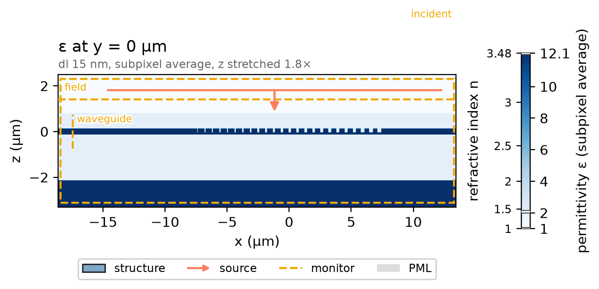
Geometry

One cell across the grating's width makes the run two-dimensional, as the paper's was. The layout runs along x with the silicon centred on z = 0: the first trench at x0, on the waveguide side; the beam leaning toward it from above; the waveguide readout lead before it. The box around them follows.

dl = wlen0 / (n_si * cells_per_wlen)  # the cell (µm), one across the width
theta = np.radians(theta_air)  # fibre tilt (rad)
L = (sum(L_E) + sum(L_O)) * 1e-3  # grating length (µm)
x0 = -L / 2  # the first trench
x_hit = x0 + fibre_offset  # the beam axis meets the oxide surface here
x_src = x_hit + z_source * np.tan(theta)  # and crosses the source plane here
x_mon = x0 - lead  # the waveguide readout plane
z_top = h / 2 + t_tox  # the oxide surface
z_src = z_top + z_source  # the source plane
beam_half = beam_radii * (mfd / 2) / np.cos(theta)  # the source's half-width
x_lo = x_mon - clearance  # the box, before the PML
x_hi = x_src + beam_half + clearance
z_lo = -h / 2 - t_box - clearance
z_hi = z_src + clearance / 2
over = (pml + 2) * dl  # every layer runs on through the PML

Five layers stack on z: an assumed silicon substrate, the buried oxide, the silicon, the top oxide and the air, each a ph.Box one cell wide. ph.Medium takes the paper's constant indices as permittivities, and ph.Structure gives each box its medium. The trenches are oxide boxes cut e deep, the narrowest nearest the waveguide.

si = ph.Medium(permittivity=n_si**2)
sio2 = ph.Medium(permittivity=n_sio2**2)
air = ph.Medium(permittivity=1.0)
layers = [
    (z_lo - over, z_hi + over, air),  # the air, filling the box
    (z_lo - over, -h / 2 - t_box, si),  # the substrate (assumed)
    (-h / 2 - t_box, -h / 2, sio2),  # the buried oxide
    (-h / 2, h / 2, si),  # the silicon
    (h / 2, z_top, sio2),  # the top oxide
]
structures = [
    ph.Structure(
        geometry=ph.Box(
            center_um=((x_lo + x_hi) / 2, 0.0, (z_a + z_b) / 2),
            size_um=(x_hi - x_lo + 2 * over, dl, z_b - z_a),
        ),
        medium=medium,
    )
    for z_a, z_b, medium in layers
]
x = x0
for le, lo in zip(L_E, L_O + [0]):  # a trench, then a tooth; the last ends on its trench
    trench = ph.Box(center_um=(x + le * 1e-3 / 2, 0.0, h / 2 - e / 2), size_um=(le * 1e-3, dl, e))
    structures.append(ph.Structure(geometry=trench, medium=sio2))
    x += (le + lo) * 1e-3

Simulation

The fibre is a ph.GaussianBeam of the fibre's mode-field diameter, polarised along the grating's width (the slab's TE polarisation) and tilted toward the waveguide, so its wavevector along the chip adds to the grating's and matches the guided wave. There are no ports: each ph.PowerMonitor reads the power crossing a plane, one in the slab lead from the grating and one across the beam just below the source. The field monitor records the vertical plane.

beam = ph.GaussianBeam(
    "z",
    z_src,
    mfd_um=mfd,
    direction="-",  # downward
    n=1.0,
    angle_theta_rad=theta,
    angle_phi_rad=0.0,  # leans toward -x, the waveguide side
    polarization="Ey",
    center_um=(x_src, 0.0, 0.0),
    window_sigmas=beam_radii,
)
freqs = ph.c0 / (wlen * 1e-6)  # (Hz)
guided = ph.PowerMonitor(
    name="waveguide",
    axis="x",
    position_um=x_mon,
    freqs_hz=freqs,
    center_um=(0.0, 0.0),
    size_um=(dl, 2 * half_window),
)
z_in = z_src - below_source  # the beam readout plane
incident = ph.PowerMonitor(name="incident", axis="z", position_um=z_in, freqs_hz=freqs)
field = ph.ProfileMonitor.plane("field", "y", 0.0, wlens_um=wlen0)

ph.Simulation holds the setup. ph.Domain is one cell wide and periodic along y (ph.Boundaries), with the box above along x and z and the PML outside. ph.Mesh is uniform at dl, and subpixel averaging places the 60 nm trench and the 100 nm silicon floor between grid lines.

sim = ph.Simulation(
    domain=ph.Domain(period_um=(None, dl, None), extent_um=(x_hi - x_lo, None, z_hi - z_lo)),
    mesh=ph.Mesh(dl_um=dl),
    background=air,
    boundaries=ph.Boundaries(y="periodic"),  # the one-cell width repeats
    subpixel=True,
    pml_num_layers=pml,
    structures=structures,
    wlens_um=wlen,  # wavelengths read out
    source=beam,
    monitors=[guided, incident, field],
    run=ph.RunSpec(shutoff=shutoff, dft_shutoff=dft_shutoff),
)
sim.plot_index(y=0.0)
plt.show()

ph.run_local runs the solver on this computer; ph.cloud.run_quoted runs it on a cloud GPU.

data = ph.run_local(sim, quiet=True)
# On a cloud GPU instead, with GPU and SOLVER from your closed-test guide:
# data = ph.cloud.run_quoted(sim, device=GPU, solver=SOLVER)

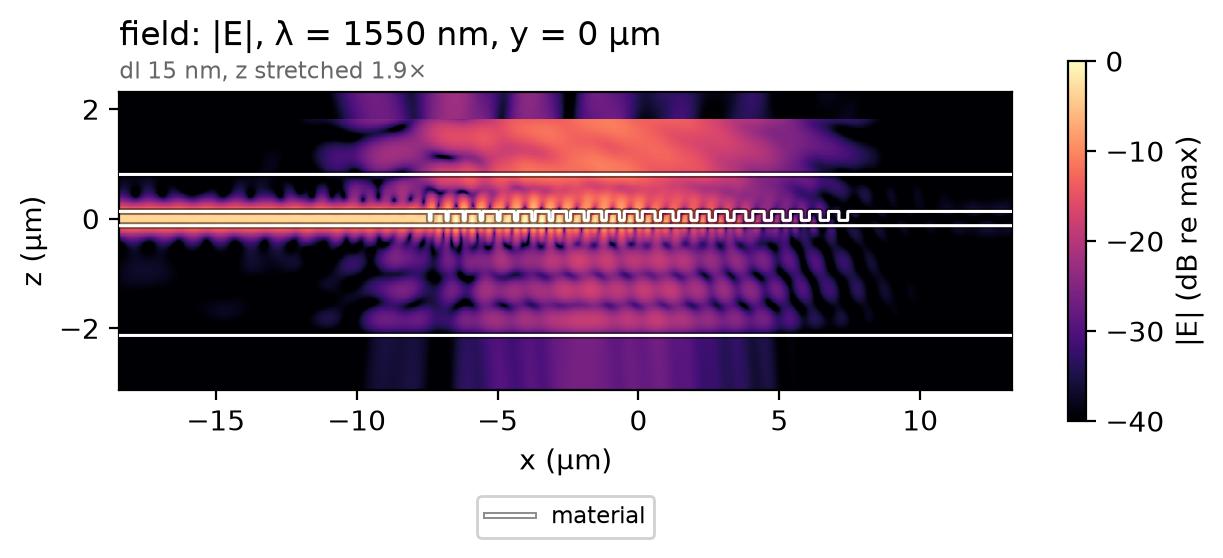
Field

The beam comes down leaning toward -x. Each trench scatters a share of it into the slab, the shares add in phase, and the guided wave leaves toward the readout. The scale is in decibels so that the beam, far weaker than the guided wave on this one cell, stays visible.

data.plot_field("field", field="E", y=0.0, scale="db")
plt.show()

Result

Coupling efficiency is the guided power over the beam's power, as the paper defines it. The beam's power comes from the same simulation with the chip removed, so the source's normalisation cancels. Both monitors count power along their axis: the guided power flows toward -x, the beam's toward -z.

empty = ph.run_local(sim.with_changes(structures=structures[:1]), quiet=True)  # the beam alone
P_guided = -data["waveguide"].values.ravel()  # flux toward -x
P_incident = -empty["incident"].values.ravel()  # flux toward -z
ce_db = 10 * np.log10(P_guided / P_incident)  # coupling efficiency (dB)

The markers are the paper's own 2D FDTD curve from its Fig. 5, one point in four, plus its peak and the points either side of each 1 dB edge. The 1 dB bandwidth is read between the two wavelengths where the efficiency falls 1 dB below its peak.

# paper-data: marchetti2017_fig5
# Fig. 5 2D FDTD, 1 in 4 points + peak and 1 dB edges; CC BY 4.0, doi:10.1038/s41598-017-16505-z
# fmt: off
paper_wlen_nm = [1502.0, 1506.0, 1510.0, 1514.0, 1518.0, 1522.0, 1526.0, 1530.0, 1533.0, 1534.0,
                 1538.0, 1542.0, 1546.0, 1549.0, 1550.0, 1554.0, 1558.0, 1562.0, 1565.0, 1566.0,
                 1570.0, 1574.0, 1578.0, 1582.0, 1586.0, 1590.0, 1594.0, 1598.0]
paper_ce_db = [-9.98, -8.715, -7.199, -5.884, -4.729, -3.76, -2.912, -2.229, -1.812, -1.687,
               -1.275, -0.996, -0.843, -0.793, -0.803, -0.879, -1.062, -1.419, -1.709, -1.802,
               -2.354, -3.002, -3.775, -4.659, -5.673, -6.792, -8.047, -9.393]
# fmt: on
ph.viz.plot_comparison(
    wlen * 1e3,
    ce_db,
    reference={"x": paper_wlen_nm, "y": paper_ce_db, "label": "paper, Fig. 5, 2D FDTD"},
    stated=(paper_peak_meas_db, "paper, stated (best measured peak)"),
    ylabel="coupling efficiency (dB)",
    ylim=(-5, 0),
)
plt.show()
i_pk = int(np.argmax(ce_db))  # the 1 dB edges, interpolated either side of the peak
edge_lo = np.interp(ce_db[i_pk] - 1.0, ce_db[: i_pk + 1], wlen[: i_pk + 1]) * 1e3
edge_hi = np.interp(ce_db[i_pk] - 1.0, ce_db[i_pk:][::-1], wlen[i_pk:][::-1]) * 1e3
ce_1550 = ce_db[int(np.argmin(np.abs(wlen - wlen0)))]
print(
    f"at 1550 nm {ce_1550:.2f} dB (paper {paper_peak_db}) | "
    f"1 dB bandwidth {edge_hi - edge_lo:.1f} nm (paper {paper_bw_nm})"
)

output

at 1550 nm -0.84 dB (paper -0.8) | 1 dB bandwidth 33.7 nm (paper 32.8)

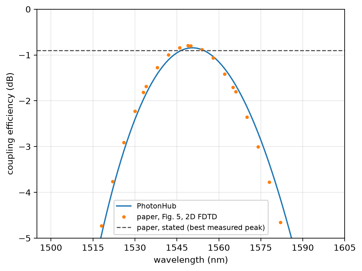
At 30 cells per wavelength the coupling efficiency reads -0.84 dB at 1550 nm; converged, -0.84 dB; the paper's 2D FDTD, -0.8 dB. The run uses a uniform mesh of 30 cells per wavelength in the silicon, one cell wide, subpixel averaging on, constant indices, 12 PML layers along x and z and no symmetry plane.