Vertically emitting photonic-crystal cavity

A photonic crystal is a material patterned with a regular lattice of holes; etched into a thin silicon membrane, the lattice stops a band of wavelengths from travelling in the plane. Leave out three holes in a row, an L3 defect, and light in that band is trapped in the gap, in about a cubic wavelength: an optical cavity. Its quality factor Q measures how long it stores light, the resonance wavelength divided by the resonance's width; such cavities reach a Q of a million in simulation and a few hundred thousand on fabricated chips. A plain L3 cavity leaks light at wide angles, so a lens above the chip collects little of it. Moving and resizing every hole around the defect steers the leakage straight up while keeping Q high. An array of such cavities, each tuned separately, then shapes a light beam pixel by pixel: a spatial light modulator. The figures of merit are Q, the resonance wavelength and the share of the emitted light within a small angle of the surface normal.

This notebook builds the published design of Panuski et al., Nat. Photon. 16, 834 (2022), rings it down, and reads its resonance and the beam it sends upward: 1559.0 nm, against the paper's 1550 nm design and the 1553 to 1562 nm its fabricated arrays were measured at. 48 % of the escaping light leaves within 10° of the surface normal, read at 12 cells per lattice constant on one mesh and not shown converged.

Parameters

The design numbers are the paper's, then its stated results; the holes come from the published design's table. The mesh has 12 cells per lattice constant. The 3 ps ring-down fixes the resonance but is under a hundredth of the photon lifetime at this Q, so the fit gives Q to its order only. The pulse reaches the mode and stays inside the band the crystal blocks. The PML sits 1.6 µm, about a wavelength, above and below the membrane, and the mode's three mirror planes cut the run to one eighth.

import json

import matplotlib.pyplot as plt
import numpy as np

import photonhub as ph
from photonhub.analysis import ResonanceAnalysis, far_field, select_resonances

# design, the paper's Fig. 3a, Fig. 4 and Sec. IV
a = 0.400  # lattice constant (µm), as in the hole table
t_slab = 0.220  # silicon membrane thickness (µm)
n_periods = 32  # cavity array period, in lattice constants
wlen0 = 1.550  # design wavelength (µm)
paper_q = 8e5  # paper, Fig. 4: simulated Q
paper_q_measured = 5.7e5  # paper, Fig. 4: measured Q
paper_wlen_measured_nm = (1553.0, 1562.0)  # paper: arrays measured (nm)

# simulation choices
cells_per_a = 12  # mesh cells per lattice constant
record_ps = 3.0  # ring-down recorded (ps)
fwidth_hz = 1e13  # pulse bandwidth (Hz)
z_clear = 1.6  # membrane to PML, above and below (µm)
pml = 12  # PML layers
symmetry = (1, -1, 1)  # the mode's three mirror planes
samples_per_period = 16  # probe samples per optical period
map_size = (8.0, 6.8)  # mid-plane field map, x and y (µm)
escape_gap = 0.15  # escape plane above the membrane (µm)
collect_deg = 10.0  # collection half-angle read out (degrees)

f0 = ph.c0 / (wlen0 * 1e-6)  # design frequency (Hz)
wlen = np.linspace(wlen0 - 0.005, wlen0 + 0.025, 21)  # field wavelengths (µm)

Geometry

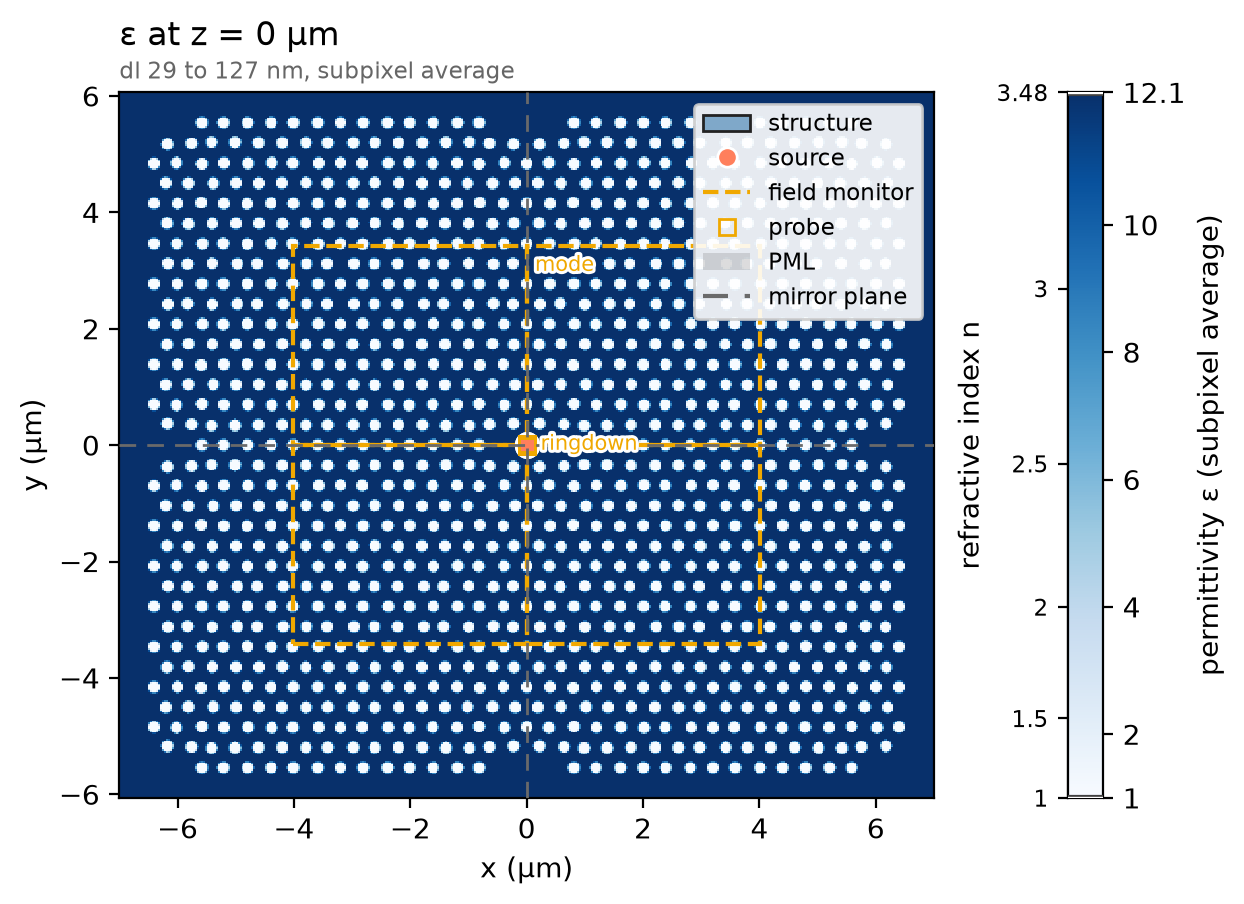
The design is a table of hole centres and radii for one quadrant of the mirror-symmetric unit cell; reflecting it across both axes gives the whole cell. The membrane is one ph.Box that runs out past every wall, and each hole is a ph.Cylinder of air through it, a ph.Medium of permittivity 1; the three holes missing at the origin are the L3 defect.

quadrant = json.load(open("refs/panuski2022_holes.json"))["holes"]  # x, y, r (µm), one quadrant
holes = sorted(
    {
        (round(sx * x, 9), round(sy * y, 9), r)
        for x, y, r in quadrant
        for sx in (-1, 1)
        for sy in (-1, 1)
    }
)  # the whole cell, each hole once
span = 4 * n_periods * a  # the membrane runs past every wall (µm)
membrane = ph.Structure(
    geometry=ph.Box(center_um=(0.0, 0.0, 0.0), size_um=(span, span, t_slab)),
    medium=ph.materials.Si,
)
air = ph.Medium(permittivity=1.0)
etch = [
    ph.Structure(
        geometry=ph.Cylinder(axis="z", center_um=(x, y, 0.0), radius_um=r, length_um=t_slab),
        medium=air,
    )
    for x, y, r in holes
]
structures = [membrane] + etch

Simulation

A y-polarised ph.PointDipole beside the cavity centre, driven by a short ph.GaussianPulse, rings the mode. With no ports, there is no mode window to size. A ph.TimeMonitor at the same point records the ring-down about 16 times per optical period, a step count set by the solver's time step.

pulse = ph.GaussianPulse(freq0_hz=f0, fwidth_hz=fwidth_hz)
dl = a / cells_per_a  # cell along x (µm)
dy = dl * np.sqrt(3) / 2  # cell along y, one row spacing per cells_per_a (µm)
dz = wlen0 / (ph.materials.Si.n(wlen0) * cells_per_a)  # finest cell along z (µm)
dt = 0.99 * min(dl, dy, dz) * 1e-6 / (ph.c0 * np.sqrt(3))  # the time step it sets (s)
interval = max(1, int(1 / (f0 * samples_per_period * dt)))  # steps per sample
point = (0.0, 0.5 * dy, 0.0)  # half a row off the centre (µm)
source = ph.PointDipole(center_um=point, polarization="Ey", source_time=pulse)
ringdown = ph.TimeMonitor(name="ringdown", center_um=point, fields=("Ey",), interval_steps=interval)

Two ph.ProfileMonitors record a comb of wavelengths, since the resonance is known only after the fit: one on the mid-plane for the mode, one just above the membrane for the light escaping upward. Their ph.Apodization opens after the pulse.

t_start = 2 * pulse.source_end_time_s  # the pulse is over (s)
apodization = ph.Apodization(
    start_s=t_start, end_s=record_ps * 1e-12 - 2 * t_start, width_s=0.5 * t_start
)
mode = ph.ProfileMonitor.plane(
    "mode",
    "z",
    0.0,
    size_um=(*map_size, 0.0),
    center_um=(0.0, 0.0, 0.0),
    wlens_um=wlen,
    fields=("Ex", "Ey", "Ez"),
    apodization=apodization,
)
escape = ph.ProfileMonitor.plane(
    "escape",
    "z",
    t_slab / 2 + escape_gap,
    wlens_um=wlen,
    fields=("Ex", "Ey", "Hx", "Hy"),
    apodization=apodization,
)

ph.Simulation holds the setup. ph.Domain spans one array period in x and y and z_clear above and below. ph.Mesh puts cells_per_a cells to a lattice constant along x and to a row spacing along y, so every hole meets the mesh alike, and grades z; subpixel averaging smooths the hole walls. The run records a fixed ring-down.

sim = ph.Simulation(
    domain=ph.Domain(
        extent_um=((n_periods + 1) * a, (n_periods + 1) * a * np.sqrt(3) / 2, None),
        clearance_um=(None, None, z_clear),
    ),
    mesh=ph.Mesh(dl_um=(dl, dy, None), cells_per_wlen=cells_per_a),
    run=ph.RunSpec(run_time_s=record_ps * 1e-12, shutoff=0.0),
    pml_num_layers=pml,
    symmetry=symmetry,
    structures=structures,
    sources=[source],
    monitors=[ringdown, mode, escape],
    wlen0_um=wlen0,
)
sim.plot_index(z=0.0)
plt.show()

ph.run_local runs the solver on this computer; ph.cloud.run_quoted runs it on a cloud GPU.

data = ph.run_local(sim, quiet=True)
# On a cloud GPU instead, with GPU and SOLVER from your closed-test guide:
# data = ph.cloud.run_quoted(sim, device=GPU, solver=SOLVER)

Field

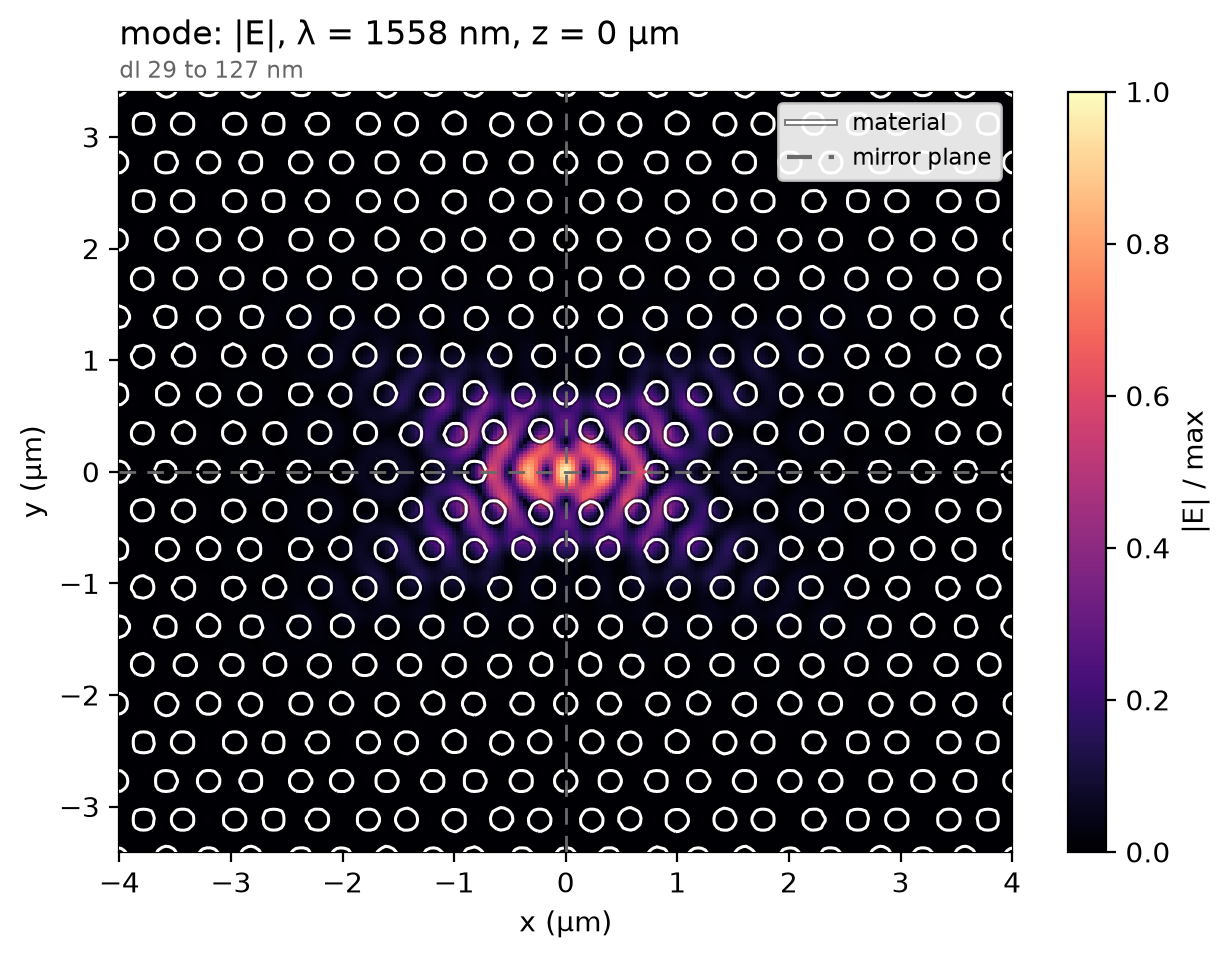
The cavity rings where its geometry puts it, not at the design point, so the profile is read at the recorded wavelength holding the most field. On the membrane's mid-plane the field is held in the three-hole defect and fades into the crystal around it.

total = np.abs(data["mode"]).sum(("component", "x", "y", "z"))  # |E| summed per wavelength
f_map = float(total.idxmax("f"))  # the recorded frequency nearest the resonance (Hz)
data.plot_field("mode", field="E", z=0.0, freq=f_map)
plt.show()

Result

The resonance and Q come from fitting the decaying poles of the ring-down after the pulse, within 10 % of the design frequency.

ring = data["ringdown"]
ts = np.asarray(ring.coords["t"].values)
ey = np.asarray(ring.sel(component="Ey").values).ravel()[ts >= t_start]
band = (0.9 * f0, 1.1 * f0)
poles = ResonanceAnalysis(freq_window=band, init_num_freqs=100)
found = poles.run_raw_signal(ey, float(ts[1] - ts[0]))
found = select_resonances(found, freq_window=band, sort_by="amplitude").isel(freq=0)
f_res, q = float(found.coords["freq"].values), float(found["Q"].values)
low, high = paper_wlen_measured_nm
print(
    f"resonance {ph.c0 / f_res * 1e9:.1f} nm (paper: {wlen0 * 1e3:.0f} nm by design, "
    f"{low:.0f} to {high:.0f} nm measured) | Q about {q:.0e} "
    f"(paper: {paper_q:.1e} simulated, {paper_q_measured:.1e} measured)"
)

output

resonance 1559.0 nm (paper: 1550 nm by design, 1553 to 1562 nm measured) | Q about 6e+05 (paper: 8.0e+05 simulated, 5.7e+05 measured)

Projecting the plane above the membrane onto the upper half space gives the emitted pattern; the curve is the share of the escaping light within a given half-angle of the normal, what a lens above the cavity gathers. The paper's own figure of merit, the light in the array's zeroth diffraction order, belongs to the infinite array, not one cavity, and is not compared.

theta = np.radians(np.linspace(0.0, 89.0, 90))
phi = np.radians(np.arange(0.0, 360.0, 10.0))
pattern = far_field(
    data, "escape", theta=theta, phi=phi, axis="z", simulation=sim, freqs_hz=[f_map]
)
intensity = pattern.dataset["intensity"].isel(f=0).values
share = np.cumsum((intensity * np.sin(theta)[:, None]).sum(axis=1))
ph.viz.plot_comparison(
    np.degrees(theta),
    share / share[-1],
    xlabel="collection half-angle (deg)",
    ylabel="share of the escaping light",
    ylim=(0.0, 1.0),
)
plt.show()
collected = share[np.searchsorted(np.degrees(theta), collect_deg)] / share[-1]
print(f"{collected:.0%} of the escaping light within {collect_deg:.0f} deg of the normal")

output

48% of the escaping light within 10 deg of the normal

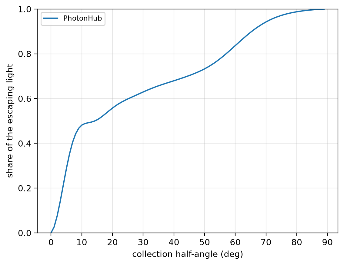
At 12 cells per lattice constant the resonance reads 1559.0 nm; at 32 cells, 1563.6 nm, not shown converged; the paper's design, 1550 nm, measured 1553 to 1562 nm. Q reads about 6 × 10⁵, its order only; the paper's, 8 × 10⁵ simulated. The 48 % within 10° is read on this one mesh too and is not shown converged. The run uses 12 cells per lattice constant in plane, graded along z, subpixel averaging on, non-dispersive silicon, 12 PML layers and three mirror planes.