Waveguide Bragg grating

A photonic chip carries light in waveguides, strips of silicon that hold light in by total internal reflection; light travels along one as a mode, a field pattern that keeps its shape. Lasers need mirrors and optical links need filters that pick out one narrow band of wavelengths. A Bragg grating is a waveguide whose width is modulated periodically along its length, and each width step reflects a little of the guided light. At the Bragg wavelength λ_B = 2 n_eff Λ, where Λ is the period and n_eff the effective index, the index the mode travels with, all the small reflections add in phase: the grating becomes a mirror for a narrow band, the stopband, and passes every other wavelength. The coupling coefficient κ (per µm) says how strongly each period reflects; a grating of length L reflects R = tanh²(κL) at its peak, so a weak corrugation needs a long grating, and the stopband widens as κ grows. The figures of merit are the peak reflection, near 1 for a mirror, the Bragg wavelength and the stopband width, from under a nanometre to tens of nanometres in silicon.

This notebook builds the strip grating of Wang et al., Opt. Express 20, 15547 (2012), a 500 x 220 nm silicon wire with 30 nm corrugations on each sidewall at a 320 nm period, 160 periods long: the peak reflection reads 0.971 at 1549 nm, against the paper's near-unity measured peak for its 2000-period gratings.

Parameters

The design numbers are the paper's Sec. 2.4 and Fig. 5; the corrugation is per sidewall. The paper's devices run 2000 periods; 160 already make a mirror near unity. The band holds the stopband and its first side lobes, sampled 0.25 nm apart to resolve the edges. The mesh is uniform. The leads are two mode widths, and the clearances keep three decay lengths of the mode's tail ahead of the PML, the absorbing layers at the walls. TE0 is mirror-symmetric about the guide's two central planes, so two symmetry planes run a quarter of the cells. Light near the stopband edges lingers in the grating, so the run continues until the field has decayed to 1e-6.

import matplotlib.pyplot as plt
import numpy as np

import photonhub as ph

# design, the paper's symbols (Sec. 2.4, Fig. 5)
w = 0.50  # strip width (µm)
h = 0.22  # silicon thickness (µm)
period = 0.320  # grating period Λ (µm)
corrugation = 0.030  # corrugation on each sidewall (µm)
paper_R_min = 0.9  # paper, Sec. 3: peak reflection above this

# simulation choices
n_periods = 160  # periods; the paper's devices run 2000
periods_sweep = (40, 80)  # shorter gratings of the sweep
wlen_min = 1.534  # band start (µm)
wlen_max = 1.562  # band end (µm)
n_wlen = 113  # wavelengths read out, 0.25 nm apart
cells_per_wlen = 12  # mesh cells per wavelength in silicon
lead = 1.0  # straight guide before each port (µm)
clearance = 0.8  # silicon edge to PML, in plane (µm)
clearance_z = 0.8  # core to PML, above and below (µm)
pml = 12  # PML layers
symmetry = (0, -1, 1)  # TE0's Ey is even across y = 0 and z = 0
shutoff = 1e-6  # field decay that ends the run
dft_shutoff = 0.0  # 0 = no spectrum-settling check

wlen = np.linspace(wlen_min, wlen_max, n_wlen)  # wavelengths (µm)
wlen0 = 0.5 * (wlen_min + wlen_max)  # band centre (µm)
f0 = ph.c0 / (wlen0 * 1e-6)  # band-centre frequency (Hz)

Geometry

The grating is one ph.Polygon, an outline in the chip plane extruded through the silicon: a lead, then a wide and a narrow half per period on both sidewalls alike, then a lead. ph.Structure makes it silicon. The sweep redraws it with fewer periods, so it is a function of the number of periods.

def grating(periods):
    L = periods * period  # the grating's length (µm)
    reach = L / 2 + lead  # the grating's centre to each port plane (µm)
    sides = []
    for sign in (-1, 1):  # the lower sidewall, then the upper
        edge = [(-reach, sign * w / 2), (-L / 2, sign * w / 2)]  # the input lead
        wide = sign * (w / 2 + corrugation)
        narrow = sign * (w / 2 - corrugation)
        for i in range(periods):  # a wide half, then a narrow half
            x0 = -L / 2 + i * period  # the period's start
            mid = x0 + period / 2  # its step from wide to narrow
            edge += [(x0, wide), (mid, wide), (mid, narrow), (x0 + period, narrow)]
        sides.append(edge + [(L / 2, sign * w / 2), (reach, sign * w / 2)])  # the output lead
    outline = sides[0] + sides[1][::-1]  # counter-clockwise
    shape = ph.Polygon(axis="z", vertices_um=outline, slab_bounds_um=(-h / 2, h / 2))
    return [ph.Structure(geometry=shape, medium=ph.materials.Si)]


structures = grating(n_periods)

Simulation

A ph.Port is a plane across a guide: its centre, the axis the light travels along, and the guide's width and thickness. in launches TE0 and reads its plane twice, forward for the launched power and backward for the reflected power; through reads what passes. The SDK sizes the window the mode is read in so the mode is 30 dB down at its edge, with a 20 % margin.

arm = n_periods * period / 2 + lead  # the grating's centre to each port plane (µm)
ports = [
    ph.Port("in", (-arm, 0.0, 0.0), "x", w, thickness_um=h),  # launch, reflection
    ph.Port("through", (arm, 0.0, 0.0), "x", w, thickness_um=h),  # transmission
]

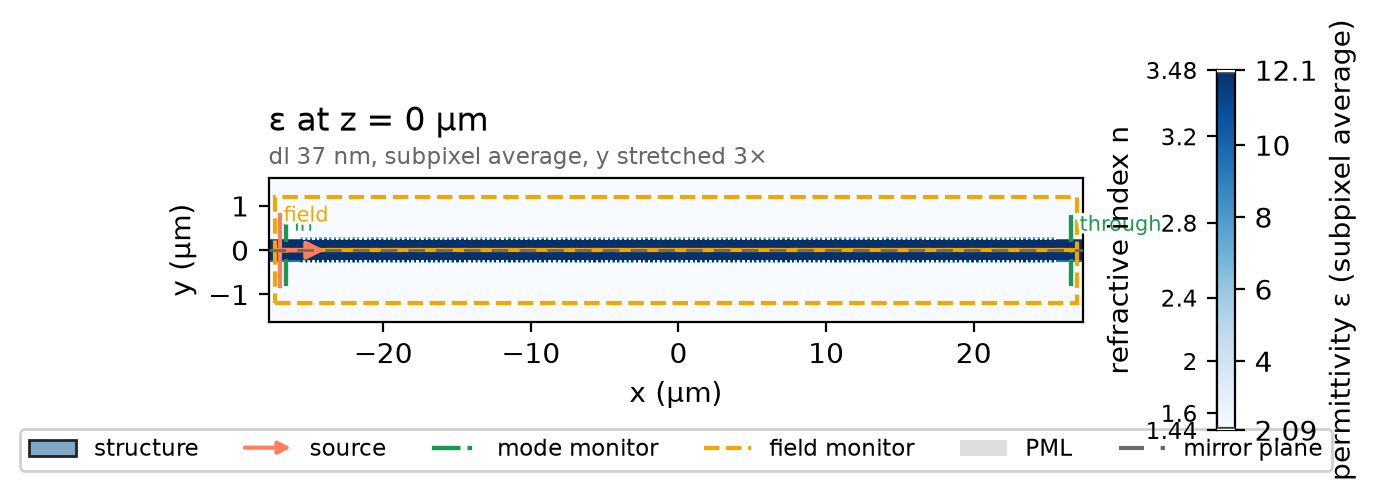
ph.Simulation holds the setup. ph.Domain fits the box around the grating and continues each guide through the PML. ph.Mesh sets cells_per_wlen cells per wavelength in the silicon, uniform here; each 30 nm tooth, smaller than a cell, sits under subpixel averaging. The field monitor records the chip plane at the band centre.

field = ph.ProfileMonitor.plane("field", "z", 0.0, wlens_um=wlen0)  # the chip plane
sim = ph.Simulation(
    domain=ph.Domain(clearance_um=(clearance, clearance, clearance_z)),
    mesh=ph.Mesh(cells_per_wlen=cells_per_wlen, uniform=True),
    background=ph.materials.SiO2,  # oxide cladding
    pml_num_layers=pml,
    structures=structures,
    symmetry=symmetry,
    wlens_um=wlen,  # wavelengths read out at the ports
    ports=ports,
    source="in",  # the port that launches TE0
    run=ph.RunSpec(shutoff=shutoff, dft_shutoff=dft_shutoff),
    monitors=[field],
)
sim.plot_index(z=0.0)
plt.show()

ph.run_local runs the solver on this computer; ph.cloud.run_quoted runs it on a cloud GPU. The outputs on this page come from a GPU run of this exact simulation.

data = ph.run_local(sim, quiet=True)
# On a cloud GPU instead, with GPU and SOLVER from your closed-test guide:
# data = ph.cloud.run_quoted(sim, device=GPU, solver=SOLVER)

Field

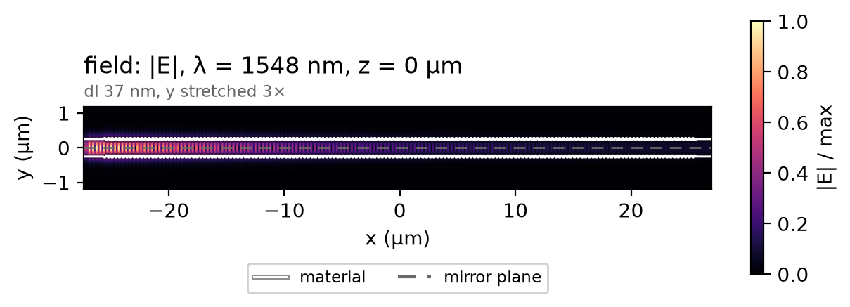
Inside the stopband, incident and reflected waves stand on the input side; the field decays into the grating over a few penetration depths, and little reaches the output. The other quarters mirror the one that ran.

data.plot_field("field", field="E", z=0.0)
plt.show()

Result

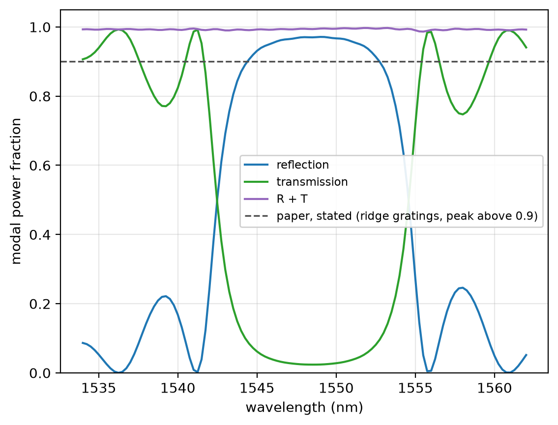
Reflection is the input plane read backward over itself read forward; transmission is the through port's power over the launched power. R + T shows how much of the power is accounted for; the rest leaves the guide. The dashed line is the peak reflection the paper states for its ridge gratings; its strip gratings measure near unity (Fig. 8), in spectra its licence keeps out of this notebook.

R = data.reflection("in")  # modal power sent back, over the launched power
T = data.transmission("through")  # modal power through the grating
ph.viz.plot_comparison(
    R.wlen_um * 1e3,
    {"reflection": R, "transmission": T, "R + T": R + T},
    stated=(paper_R_min, "paper, stated (ridge gratings, peak above 0.9)"),
    ylabel="modal power fraction",
    ylim=(0, 1.05),
)
plt.show()
peak = R.isel(f=int(np.argmax(R.values)))  # the stopband peak
kappa = float(np.arctanh(np.sqrt(peak)) / (n_periods * period))  # from R = tanh²(κL)
wlen_peak = float(peak.wlen_um) * 1e3  # (nm)
balance = float(peak + T.sel(f=peak.f))  # R + T at the peak
print(
    f"peak reflection {float(peak):.4f} at {wlen_peak:.2f} nm | R + T there {balance:.4f} | "
    f"κ = {kappa:.4f} /µm, penetration depth {1 / kappa:.1f} µm"
)

output

peak reflection 0.9713 at 1549.00 nm | R + T there 0.9954 | κ = 0.0481 /µm, penetration depth 20.8 µm

At 12 cells per wavelength the peak reflection reads 0.971 at 1549 nm; at 20 cells, 0.976, not shown converged; the paper's measurement, near unity (Fig. 8). The run uses a uniform mesh of 12 cells per wavelength in the silicon, subpixel averaging on, non-dispersive silicon and oxide, 12 PML layers and two symmetry planes through the guide axis.

Sweep

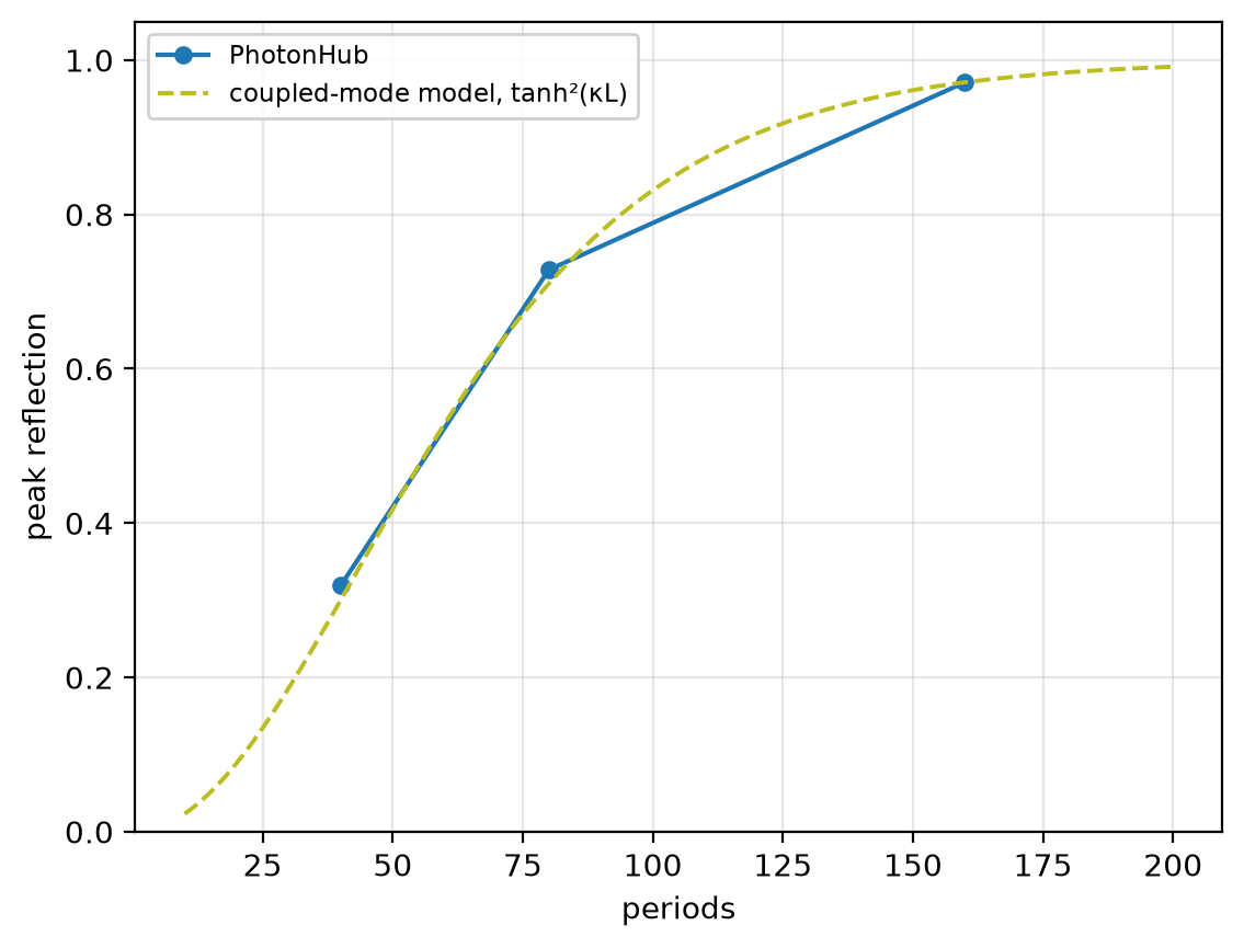
Coupled-mode theory ties κ to the cross-section, not the length, so one κ must fit every length through R = tanh²(κL). Each point is a full run of a shorter grating with the ports at its ends; the dashed curve is the model with κ from the 160-period run.

peaks = []
for n in periods_sweep:
    reach = n * period / 2 + lead  # the ports move to the grating's ends
    moved = [
        ph.Port("in", (-reach, 0.0, 0.0), "x", w, thickness_um=h),
        ph.Port("through", (reach, 0.0, 0.0), "x", w, thickness_um=h),
    ]
    out = ph.run_local(sim.with_changes(structures=grating(n), ports=moved), quiet=True)
    peaks.append(float(out.reflection("in").max()))
peaks.append(float(peak))
N = np.array([*periods_sweep, n_periods])  # periods of the three runs
N_curve = np.arange(10, 201)  # periods on the model curve
ph.viz.plot_comparison(
    N,
    np.array(peaks),
    model=(N_curve, np.tanh(kappa * N_curve * period) ** 2, "coupled-mode model, tanh²(κL)"),
    xlabel="periods",
    ylabel="peak reflection",
    ylim=(0, 1.05),
)
plt.show()
kappas = [np.arctanh(np.sqrt(r)) / (m * period) for m, r in zip(N, peaks)]
print(" | ".join(f"{m} periods: R {r:.3f}, κ {k:.4f} /µm" for m, r, k in zip(N, peaks, kappas)))

output

40 periods: R 0.319, κ 0.0500 /µm | 80 periods: R 0.728, κ 0.0495 /µm | 160 periods: R 0.971, κ 0.0481 /µm