Broadband directional coupler

A photonic chip often splits light between two paths, for example to feed the two arms of an interferometer. Light travels in waveguides, strips of silicon in glass, as a mode, a field pattern that keeps its shape. A directional coupler runs two waveguides side by side a few hundred nanometres apart: the mode of one guide leaks into the other and back, so the coupler's length sets how much power crosses over. The fraction that leaves through the crossed guide is the splitting ratio, one half for a 50/50 splitter. A plain coupler holds that split over only a few tens of nanometres of wavelength, because the leak grows with the wavelength. This design puts a phase-control section between two identical couplers: two guides of different widths, whose light travels at different speeds and gains a wavelength-dependent phase difference that offsets the couplers' drift. The figures of merit are the splitting ratio across the band, ideally within a few hundredths of one half, and the width of the band that holds it, near 100 nm for a broadband design against 20 to 40 nm for a plain coupler.

This notebook builds the asymmetric-waveguide coupler of Lu et al., Opt. Express 23, 3795 (2015) from the paper's dimensions and reads the cross-port fraction across 1500 to 1600 nm: 0.5072 at 1550 nm, inside the paper's stated 3D FDTD range of 0.5 ± 0.035 over the band.

Parameters

The design numbers are the paper's TE 50/50 design. As drawn in its Fig. 1, the narrow guide is assumed to narrow toward the gap and the wide guide to widen away from it. The band is the paper's simulated range. The split is decided across the guides, so the mesh is graded: 20 cells per 1500 nm wavelength in silicon along the coupler, and 10 nm cells across the guides and through the slab. TE0 is even about the slab's mid-plane, so a mirror plane there halves the run.

import matplotlib.pyplot as plt
import numpy as np

import photonhub as ph

# design, the paper's Fig. 1 and Sec. 2.3
w = 0.50  # guide width in the symmetric couplers (µm)
h = 0.22  # silicon thickness (µm)
g1 = 0.20  # gap in the symmetric couplers (µm)
L1 = 12.4  # length of each symmetric coupler (µm)
w1 = 0.60  # wide guide in the phase section (µm)
w2 = 0.40  # narrow guide in the phase section (µm)
L2 = 4.6  # phase section (µm); 20 nm moves the split 0.01
L_t = 1.0  # linear taper between the sections (µm)
R = 5.0  # radius of the 90° port bends (µm)
paper_split = 0.5  # paper: the design's cross-port fraction
paper_dev = 0.035  # paper, stated: 3D FDTD within this of 0.5

# simulation choices
wlen_min = 1.50  # band start (µm)
wlen_max = 1.60  # band end (µm)
n_wlen = 21  # wavelengths read out
cells_at_wlen_min = 20  # cells per 1500 nm wavelength, in silicon
dl_gap = 0.010  # cell across the guides and the slab (µm)
lead = 1.5  # straight guide from each bend to its port (µm)
clearance = 1.25  # silicon edge to PML, in plane (µm)
clearance_z = 1.0  # core to PML, above and below (µm)
pml = 12  # PML layers
symmetry = (0, 0, 1)  # mirror plane through the slab's middle
transits = 4  # longest run, in transits of the device
shutoff = 1e-5  # field decay that ends the run

wlen = np.linspace(wlen_min, wlen_max, n_wlen)  # wavelengths (µm)
wlen0 = 0.5 * (wlen_min + wlen_max)  # band centre (µm)
f0 = ph.c0 / (wlen0 * 1e-6)  # band-centre frequency (Hz)
cells_per_wlen = cells_at_wlen_min * wlen0 / wlen_min  # the same, counted at wlen0

Geometry

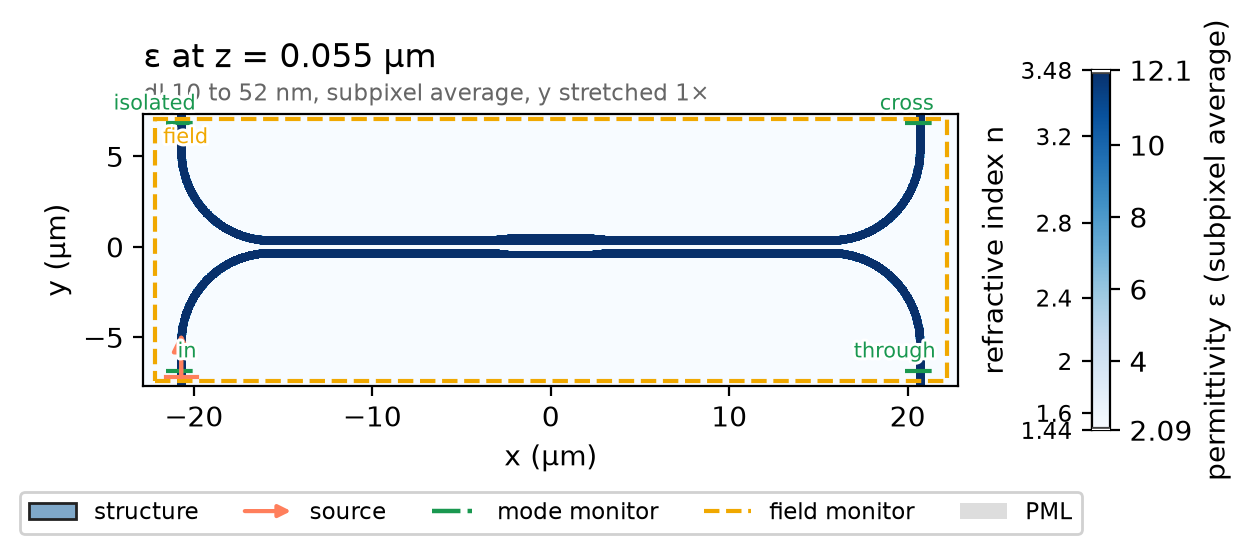
Each waveguide body is a ph.Polygon, an outline in the chip plane (vertices_um) extruded through the silicon (slab_bounds_um), with one straight edge: w wide in both couplers, w1 or w2 in the phase section, linear tapers between. The coupler is centred on the origin, and the lower guide is the input.

L_body = 2 * L1 + 2 * L_t + L2  # straight coupler body (µm)
xl = -L_body / 2  # body's left end (µm)
xr = L_body / 2  # body's right end (µm)
ya = -(w + g1) / 2  # lower (input) guide's axis (µm)
yb = (w + g1) / 2  # upper guide's axis (µm)
x_steps = [xl, xr, xr, xr - L1, xr - L1 - L_t, xl + L1 + L_t, xl + L1, xl]
bodies = [
    ph.Polygon(
        axis="z",
        vertices_um=list(zip(x_steps, [e, e, e + w, e + w, e + wm, e + wm, e + w, e + w])),
        slab_bounds_um=(-h / 2, h / 2),
    )
    for e, wm in ((ya - w / 2, w2), (yb - w / 2, w1))  # straight lower edge, middle width
]

A 90° bend on each end, a ph.Cylinder sector with outer and inner radii one guide width apart, turns each guide toward a port, and a ph.Box lead carries it there. ph.Structure gives every shape the library's silicon.

bends = [
    ph.Cylinder(
        axis="z",
        center_um=(cx, cy, 0.0),
        radius_um=R + w / 2,
        inner_radius_um=R - w / 2,
        length_um=h,
        angle_start_rad=q * np.pi / 2,
        angle_stop_rad=q * np.pi / 2 + np.pi / 2,
    )
    for cx, cy, q in ((xl, ya - R, 1), (xl, yb + R, 2), (xr, ya - R, 0), (xr, yb + R, 3))
]
y_lo = ya - R - lead  # lower port planes (µm)
y_hi = yb + R + lead  # upper port planes (µm)
leads = [
    ph.Box(center_um=(x, (y0 + y1) / 2, 0.0), size_um=(w, y1 - y0, h))
    for x in (xl - R, xr + R)
    for y0, y1 in ((y_lo, ya - R), (yb + R, y_hi))
]
structures = [ph.Structure(geometry=s, medium=ph.materials.Si) for s in bodies + bends + leads]

Simulation

A ph.Port is a plane across a guide: its centre, the axis the light travels along, and the guide's width and thickness. TE0 is launched at in on the lower left lead and read at through (lower right), cross (upper right) and isolated (upper left). The SDK sizes the window each mode is solved and read in so the mode is 30 dB down at its edge, with a 20 % margin.

ports = [
    ph.Port("in", (xl - R, y_lo, 0.0), "y", w, thickness_um=h),  # lower left
    ph.Port("through", (xr + R, y_lo, 0.0), "y", w, thickness_um=h),
    ph.Port("cross", (xr + R, y_hi, 0.0), "y", w, thickness_um=h),
    ph.Port("isolated", (xl - R, y_hi, 0.0), "y", w, thickness_um=h),
]

ph.Simulation holds the setup. ph.Domain fits the box around the device and continues each lead through the PML. ph.Mesh grades the mesh by cells_per_wlen, counted at the band centre, and a ph.MeshOverride forces dl_gap cells across the guides and through the slab. The field monitor records the plane a quarter of the way up the core.

y0 = ya - w / 2 - w  # the fine band across the guides (µm)
y1 = yb - w / 2 + w1 + w
fine = ph.MeshOverride(
    geometry=ph.Box(center_um=(0.0, (y0 + y1) / 2, 0.0), size_um=(L_body, y1 - y0, h)),
    dl_um=(None, dl_gap, dl_gap),  # across the guides and through the slab
)
field = ph.ProfileMonitor.plane("field", "z", h / 4, wlens_um=wlen0)  # a quarter up the core
sim = ph.Simulation(
    domain=ph.Domain(clearance_um=(clearance, clearance, clearance_z)),
    mesh=ph.Mesh(cells_per_wlen=cells_per_wlen, refine=(fine,)),
    background=ph.materials.SiO2,  # oxide cladding
    pml_num_layers=pml,
    structures=structures,
    symmetry=symmetry,
    wlens_um=wlen,  # wavelengths read out at the ports
    ports=ports,
    source="in",  # the port that launches TE0
    run=ph.RunSpec(transits=transits, shutoff=shutoff),
    monitors=[field],
)
sim.plot_index(z=h / 4)
plt.show()

ph.run_local runs the solver on this computer; ph.cloud.run_quoted runs it on a cloud GPU. The outputs on this page come from a GPU run of this exact simulation.

data = ph.run_local(sim, quiet=True)
# On a cloud GPU instead, with GPU and SOLVER from your closed-test guide:
# data = ph.cloud.run_quoted(sim, device=GPU, solver=SOLVER)

Field

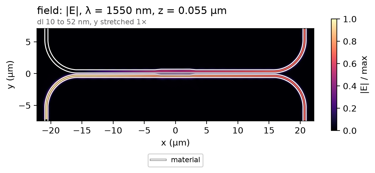
Light launched in the lower guide crosses over in the first coupler, picks up the phase section's phase, and the second coupler completes the split; at the band centre the two output leads carry equal power.

data.plot_field("field", field="E", z=h / 4)
plt.show()

Result

The observable is the paper's splitting ratio: the cross-port modal power over the sum of the cross- and through-port modal powers. The dashed lines are the range the paper states for its 3D FDTD over the band; the article's licence does not allow re-plotting its curves here.

T_through = data.transmission("through")  # through-port modal power ratio
T_cross = data.transmission("cross")  # cross-port modal power ratio
eta = T_cross / (T_cross + T_through)  # cross-port fraction of the output
ph.viz.plot_comparison(
    eta,
    stated=[
        (paper_split + paper_dev, "paper, stated (3D FDTD, upper bound)"),
        (paper_split - paper_dev, "paper, stated (3D FDTD, lower bound)"),
    ],
    ylabel="cross-port fraction of the output power",
    ylim=(0.40, 0.60),
)
plt.show()
eta_1550 = float(eta.sel(f=f0, method="nearest"))
spread = f"{float(eta.min()):.3f}-{float(eta.max()):.3f}"
print(f"cross-port fraction at 1550 nm: {eta_1550:.4f} | over the band {spread}")

output

cross-port fraction at 1550 nm: 0.5072 | over the band 0.470-0.507

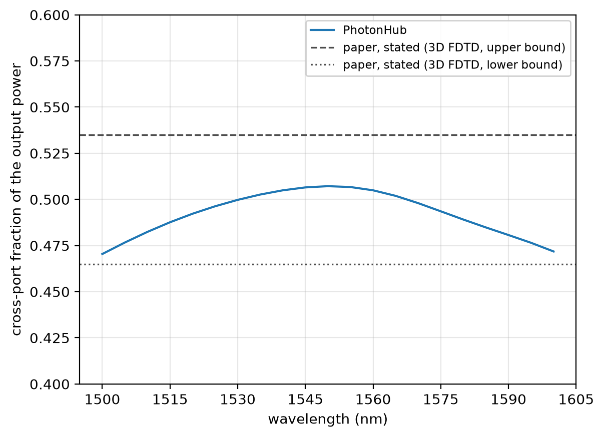
At 20 cells per wavelength along the coupler and 10 nm across it the cross-port fraction reads 0.5072 at 1550 nm, on the finest mesh run, not shown converged; the paper's 3D FDTD, within 0.035 of one half. The run uses a graded mesh with 10 nm cells across the coupler, subpixel averaging on, non-dispersive silicon and oxide, 12 PML layers and one mirror plane through the slab.