Zero-index pillar array with a bound state

Light is a wave whose phase advances as it travels, and the refractive index says how fast: in glass about one and a half times as fast as in air. At an index of zero the phase does not advance at all, so the light oscillates in step across the whole material, however large. That helps wherever many points of a circuit must stay in step, for example to feed several outputs with the same phase. No natural material has a zero index at telecom wavelengths, but a square array of silicon pillars in glass can act as one. Light crosses the array in modes, field patterns that keep their shape. At one wavelength two modes meet in a Dirac cone, a point where frequency grows linearly with the wave's spacing in every direction, and the array's index passes through zero. On a chip this mode also leaks light out of the plane. At one pillar height two field patterns inside each pillar leak with opposite phase and cancel: a bound state in the continuum. Three numbers rate the array: the wavelength of zero index, the slope of the index there, and the loss in decibels per micrometre (dB/µm).

This notebook builds 57 periods of the array of Dong et al., Light Sci. Appl. 10, 10 (2021) and reads its index from the phase advance per period: the index crosses zero at 1555.7 nm with a slope of −2.54e-3 per nm, against the paper's 1552.4 nm and −2.61e-3. There it loses 0.015 dB/µm; 1200 nm tall, without the bound state, 0.18 dB/µm.

Parameters

The design numbers and permittivities are the paper's, then its stated results. A whole number of cells per pitch makes every pillar meet the mesh alike; the gap to the PML keeps the beam's tail under 5 % of its peak. Ez is even across the mid-height, so a symmetry plane there halves the run.

import matplotlib.pyplot as plt
import numpy as np

import photonhub as ph

# design, the paper's symbols and constants
a = 0.733  # pitch of the square array (µm)
r = 0.180  # pillar radius (µm); 1 nm moves the cone 5 nm
h = 1.085  # pillar height, bound state (µm)
h_tall = 1.200  # comparison height, no bound state (µm)
eps_si = 11.7  # silicon permittivity
k_si = 2.12e-5  # silicon extinction at 1550 nm
eps_sio2 = 2.09  # oxide permittivity
n_pillars = 57  # assumed: pillars along the slab
waist = 0.8  # assumed: beam waist across the height (µm)
paper_wlen_zero = 1552.4  # paper, Fig. 5d: zero-index wavelength (nm)
paper_slope = -0.002609  # paper, Fig. 5d: index slope (1/nm)

# simulation choices
wlen_min = 1.53  # band start (µm)
wlen_max = 1.59  # band end (µm)
n_wlen = 61  # wavelengths read out
wlen0 = 1.55  # wavelength of the silicon extinction (µm)
cells_per_a = 24  # mesh cells per pitch
lead = 2.0  # oxide before and after the slab (µm)
z_gap = 1.1  # pillar end to PML (µm)
pml = 12  # PML layers
symmetry = (0, 0, -1)  # symmetry plane at mid-height
run_time = 10e-12  # longest run (s)
shutoff = 1e-5  # field decay that ends the run
dft_shutoff = 0.0  # 0 = no spectrum-settling check
trim = 6  # pillars skipped at each facet in the fits

wlen = np.linspace(wlen_min, wlen_max, n_wlen)  # wavelengths (µm)
f0 = ph.c0 / (wlen0 * 1e-6)  # frequency of the extinction (Hz)

Geometry

The slab is one row of pillars along x, centred on the origin with mid-height at z = 0; periodic walls one pitch apart repeat it into the square array. Each pillar is a ph.Cylinder along z. ph.Medium takes a permittivity, and silicon's extinction enters as a conductivity.

L = n_pillars * a  # slab length (µm)
x_pillars = [(i + 0.5) * a - L / 2 for i in range(n_pillars)]  # pillar centres (µm)
sigma_si = 4 * np.pi * f0 * ph.eps0 * np.sqrt(eps_si) * k_si  # silicon conductivity (S/m)
si = ph.Medium(permittivity=eps_si, conductivity_s_per_m=sigma_si)
sio2 = ph.Medium(permittivity=eps_sio2)
structures = [
    ph.Structure(
        geometry=ph.Cylinder(axis="z", center_um=(x, 0.0, 0.0), radius_um=r, length_um=h),
        medium=si,
    )
    for x in x_pillars
]

Simulation

The paper lights the slab with a plane wave, but here the oxide is open above and below, where a plane wave would mostly run past the pillars, so ph.GaussianBeam launches a beam flat across the row and Gaussian over the pillar height. ph.ProfileMonitors record Ez on a line through the pillar centres (axis) and on the vertical plane through the row (field). With no ports, there is no mode window to size.

dl = a / cells_per_a  # mesh cell (µm)
z_wall = h / 2 + z_gap  # PML starts here, above and below (µm)
x_src = -L / 2 - lead / 2  # source plane (µm)
beam = ph.GaussianBeam(
    "x",
    x_src,
    waist_um=(1e3, waist),  # flat along y, Gaussian along z
    polarization="Ez",
    center_um=(x_src, 0.0, 0.0),
    waist_distance_um=-lead / 2,  # focus on the first pillar
    half_v_um=z_wall - dl,  # the source stops short of the PML
)
axis = ph.ProfileMonitor(
    name="axis",
    center_um=(0.0, 0.0, 0.0),
    size_um=(L + 2 * lead, 0.0, 0.0),
    fields=("Ez",),
    freqs_hz=tuple(ph.c0 / (wlen * 1e-6)),
)
field = ph.ProfileMonitor.plane("field", "y", 0.0, wlens_um=wlen[::5], fields=("Ez",))

The domain is one pitch wide, periodic along y, with PML along x and z. The mesh is uniform, with subpixel averaging at the curved pillar walls.

sim = ph.Simulation(
    domain=ph.Domain(period_um=(None, a, None), extent_um=(L + 2 * lead, None, (-z_wall, z_wall))),
    mesh=ph.Mesh(dl_um=dl, uniform=True),
    background=sio2,
    boundaries=ph.Boundaries(y="periodic"),  # repeats the row into the array
    subpixel=True,
    pml_num_layers=pml,
    symmetry=symmetry,
    structures=structures,
    wlens_um=wlen,
    source=beam,
    monitors=[axis, field],
    run=ph.RunSpec(run_time_s=run_time, shutoff=shutoff, dft_shutoff=dft_shutoff),
)
sim.plot_index(y=0.0)
plt.show()

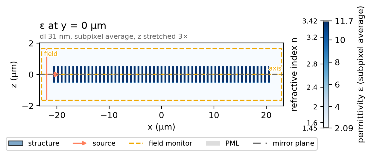
ph.run_local runs the solver on this computer; ph.cloud.run_quoted runs it on a cloud GPU. The outputs on this page come from a GPU run of this exact simulation.

data = ph.run_local(sim, quiet=True)
# On a cloud GPU instead, with GPU and SOLVER from your closed-test guide:
# data = ph.cloud.run_quoted(sim, device=GPU, solver=SOLVER)

A wave that advances by a phase φ per micrometre has the index φ / k₀. Line fits to the phase and the amplitude (in dB) of Ez at the pillar centres give φ and the decay.

inner = x_pillars[trim:-trim]


def index_and_decay(result):
    Ez = result["axis"].sel(component="Ez")
    x, f = Ez.coords["x"].values, Ez.coords["f"].values
    at = [int(np.argmin(np.abs(x - xp))) for xp in inner]
    E = Ez.transpose("f", "x", ...).values.reshape(len(f), len(x))[:, at]
    order = np.argsort(ph.c0 / f)  # by wavelength
    phase = np.unwrap(np.angle(E), axis=1).T  # phase at each pillar
    k0 = 2 * np.pi * f / ph.c0 * 1e-6  # free-space wavenumber (1/µm)
    n = (np.polyfit(inner, phase, 1)[0] / k0)[order]
    decay = -np.polyfit(inner, 20 * np.log10(np.abs(E)).T, 1)[0][order]  # dB/µm
    i = int(np.argmax(n < 0))  # the first wavelength past the crossing
    lam = (ph.c0 / f * 1e9)[order]
    return lam, n, decay, float(np.interp(0.0, [n[i], n[i - 1]], [lam[i], lam[i - 1]]))


wlen_nm, n_eff, decay_db, wlen_zero = index_and_decay(data)

Field

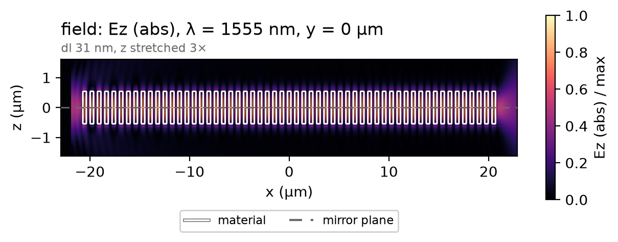
At the zero crossing every pillar oscillates in phase with the same amplitude, and the bound state lets nothing leak into the oxide.

f_planes = data["field"].coords["f"].values
f_zero = float(f_planes[np.argmin(np.abs(ph.c0 / f_planes * 1e9 - wlen_zero))])
data.plot_field("field", field="Ez", y=0.0, freq=f_zero, val="abs")
plt.show()

Result

The markers are the paper's retrieved index from its Fig. 5d. The slope is set by the group velocity of the Dirac cone.

# paper-data: dong2021_fig5d
# Fig. 5d retrieved index; CC BY 4.0, doi:10.1038/s41377-020-00436-y
# fmt: off
paper_wlen_nm = [1520.0, 1525.0, 1530.0, 1535.0, 1540.0, 1545.0, 1550.0, 1555.0, 1560.0,
                 1565.0, 1570.0, 1575.0, 1580.0, 1585.0, 1590.0, 1595.0, 1600.0]
paper_n = [0.0863, 0.0726, 0.0588, 0.0454, 0.032, 0.0186, 0.0052, -0.0076, -0.0203,
           -0.033, -0.0456, -0.0584, -0.0711, -0.0832, -0.0953, -0.1074, -0.1194]
# fmt: on
ph.viz.plot_comparison(
    wlen_nm,
    n_eff,
    reference={"x": paper_wlen_nm, "y": paper_n, "label": "paper, Fig. 5d, retrieved index"},
    ylabel="index from the phase advance per period",
    ylim=(-0.15, 0.15),
)
plt.show()
slope = np.polyfit(wlen_nm, n_eff, 1)[0]
print(
    f"zero-index wavelength: {wlen_zero:.1f} nm (paper {paper_wlen_zero} nm) | "
    f"slope {slope * 1e3:.2f}e-3 per nm (paper {paper_slope * 1e3:.2f}e-3) | "
    f"decay there {np.interp(wlen_zero, wlen_nm, decay_db):.3f} dB/µm"
)

output

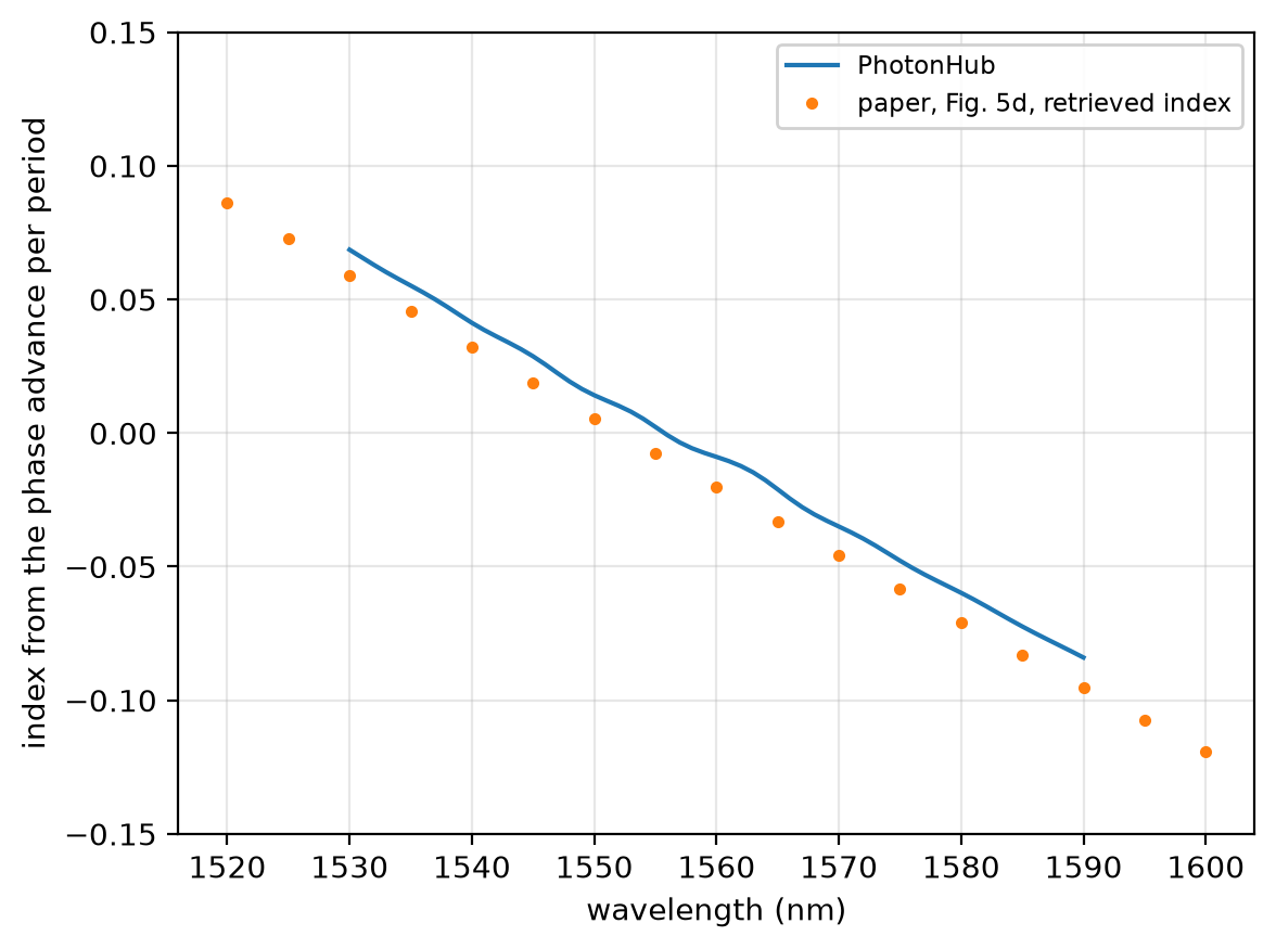
zero-index wavelength: 1555.7 nm (paper 1552.4 nm) | slope -2.54e-3 per nm (paper -2.61e-3) | decay there 0.015 dB/µm

At 24 cells per pitch the zero-index wavelength reads 1555.7 nm; at 32 cells, 1553.9 nm, not shown converged; the paper's retrieved index, 1552.4 nm. The run uses a uniform mesh of 24 cells per pitch, subpixel averaging on, non-dispersive media, 12 PML layers along x and z and one symmetry plane at mid-height.

Sweep

The paper compares the same array 1200 nm tall, without the bound state; its loss is read at its own zero-index wavelength.

structures_tall = [
    ph.Structure(
        geometry=ph.Cylinder(axis="z", center_um=(x, 0.0, 0.0), radius_um=r, length_um=h_tall),
        medium=si,
    )
    for x in x_pillars
]
data_tall = ph.run_local(sim.with_changes(structures=structures_tall), quiet=True)
_, n_tall, decay_tall, zero_tall = index_and_decay(data_tall)
print(
    f"h = {h_tall * 1e3:.0f} nm: zero-index wavelength {zero_tall:.1f} nm, decay there "
    f"{np.interp(zero_tall, wlen_nm, decay_tall):.2f} dB/µm | h = {h * 1e3:.0f} nm: "
    f"{np.interp(wlen_zero, wlen_nm, decay_db):.3f} dB/µm"
)

output

h = 1200 nm: zero-index wavelength 1571.3 nm, decay there 0.18 dB/µm | h = 1085 nm: 0.015 dB/µm