Fibre-to-chip edge coupler

Light enters a photonic chip from an optical fibre, whose core carries a round spot a few micrometres across. On the chip, light travels in waveguides: strips of a material with a high refractive index, the number that says how strongly a material slows light, set in glass. A waveguide holds a mode, a field pattern that keeps its shape, far smaller than the fibre's spot, so a fibre butted against it loses most of its light. An edge coupler narrows the waveguide to a tip at the chip's edge. A narrow guide holds its light weakly, so its mode swells into the glass until it matches the fibre's spot, then shrinks back as the guide widens. The widening must be gradual or light scatters away, and one slow taper is long; this design cascades short tapers, each as fast as its local width allows. The figure of merit is the coupling efficiency, the fraction of the fibre's power carried on in the waveguide's fundamental mode, TE0 or TM0 for the two orientations of the field; good couplers reach 80 to 95 % over a band some hundreds of nanometres wide.

This notebook builds the four-stage taper of Bhandari et al., IEEE Photonics J. 12, 6602511 (2020), puts a 4 µm fibre mode on its 200 nm tip and reads the end waveguide from 1000 to 2000 nm: 87.1 % coupling for TE0 and 90.9 % for TM0 at 1550 nm, against the paper's 93.5 % and 87.8 %.

Parameters

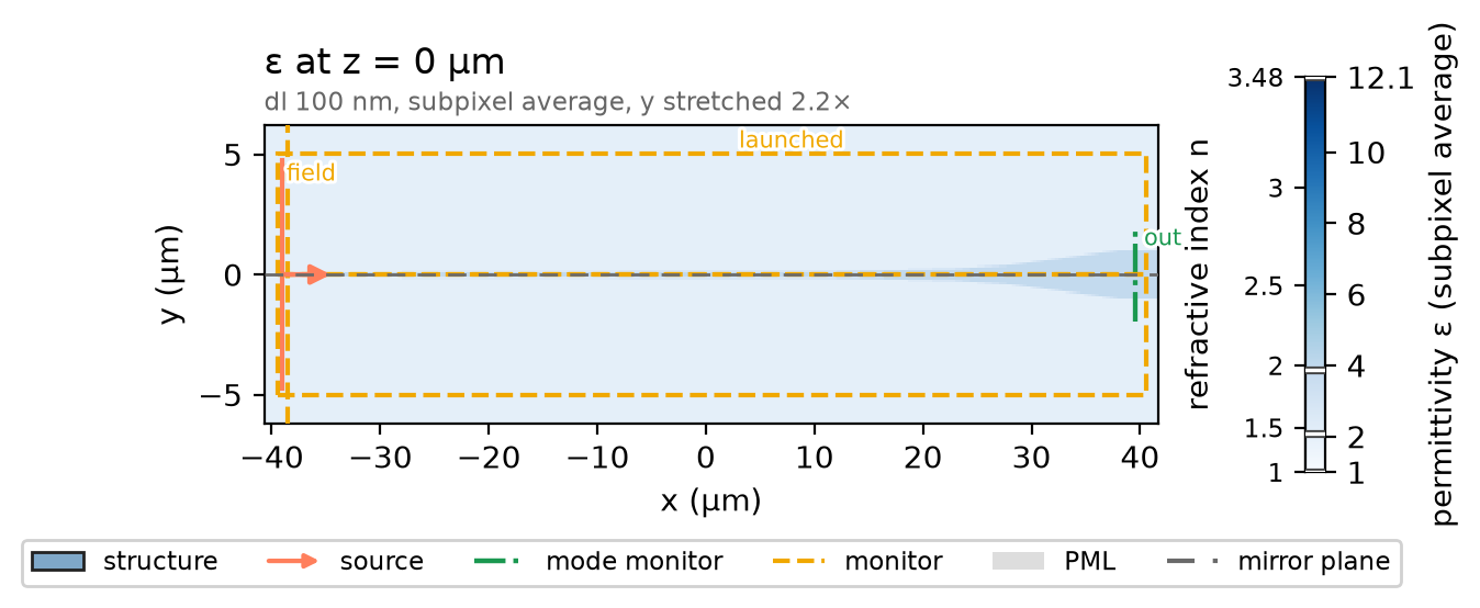
The design numbers are the paper's, with the constant indices it used; the silicon substrate's index is assumed. The band is that of its Fig. 5(a) and 8(a), in a blue and a red run per polarization: one pulse drives up to about 1.7 times its lowest frequency, and 1000 to 2000 nm spans a factor of two. A uniform 100 nm mesh treats the 200 nm tip and the taper walls alike along the whole taper. The domain reaches five mode radii beside the fibre mode. The coupler and both fundamental modes are mirror symmetric about y = 0, so a mirror plane there halves the run.

import matplotlib.pyplot as plt
import numpy as np

import photonhub as ph

# design, the paper's Sec. 2
t_core = 0.5  # silicon nitride core thickness (µm)
w_tip = 0.2  # taper tip width (µm)
w_end = 2.0  # end waveguide width (µm)
stages = ((0.3, 50.0), (0.5, 11.0), (0.8, 5.0), (2.0, 10.0))  # (width, length) (µm)
t_box = 4.0  # buried oxide under the core (µm)
t_clad = 3.0  # oxide cladding over the core (µm)
n_core = 1.97  # silicon nitride index
n_clad = 1.44  # oxide index
n_sub = 3.48  # assumed: silicon substrate index
mfd = 4.0  # fibre mode field diameter at 1550 nm (µm)

# simulation choices
wlen_min = 1.0  # band start (µm)
wlen_split = 1.4  # where the two runs meet, read by both (µm)
wlen_max = 2.0  # band end (µm)
d_wlen = 0.025  # wavelength step (µm)
dl = 0.10  # uniform mesh cell (µm)
gap = 1.0  # fibre plane to chip facet (µm)
lead = 1.5  # end waveguide before the port plane (µm)
half_y = 5.0  # domain half width (µm)
pad = 0.35  # substrate and cladding top to the PML (µm)
behind = 0.5  # fibre plane to the PML (µm)
beyond = 1.0  # port plane to the PML (µm)
overhang = 4.0  # substrate and air boxes past the PML (µm)
inset = 0.2  # beam edge inside the domain (µm)
pml = 12  # PML layers
shutoff = 1e-5  # field decay that ends the run
dft_shutoff = 0.0  # 0 = no spectrum-settling check

bands = [
    np.linspace(lo, hi, round((hi - lo) / d_wlen) + 1)
    for lo, hi in ((wlen_min, wlen_split), (wlen_split, wlen_max))
]  # wavelengths of the two runs (µm)
wlen0 = 2 / (1 / wlen_min + 1 / wlen_max)  # band centre in frequency (µm)
f0 = ph.c0 / (wlen0 * 1e-6)  # band-centre frequency (Hz)

Geometry

The taper is a ph.Polygon, an outline in the chip plane (vertices_um, an edge and its mirror image) extruded through the nitride (slab_bounds_um), centred on the origin. It starts w_tip wide at the facet, widens through the four stages and runs on through the PML as the end waveguide. Two ph.Boxes carry the rest of the stack, the silicon under the buried oxide and the air over the cladding, wider than the domain. ph.Medium takes each index as a permittivity.

length = sum(seg for _, seg in stages)  # taper length (µm)
x_facet = -length / 2  # the tip, on the chip facet (µm)
x_port = length / 2 + lead  # port plane (µm)
x_lo = x_facet - gap - behind  # domain ends along x (µm)
x_hi = x_port + beyond
z_sub = -t_box - t_core / 2  # top of the substrate (µm)
z_top = t_clad + t_core / 2  # top of the cladding (µm)
z_lo = z_sub - pad  # domain ends along z (µm)
z_hi = z_top + pad
x_stage = x_facet + np.cumsum([0.0] + [seg for _, seg in stages])  # stage ends (µm)
w_stage = [w_tip] + [w for w, _ in stages]
edge = [(x, w / 2) for x, w in zip(x_stage, w_stage)] + [(x_hi + overhang / 2, w_end / 2)]
taper = ph.Polygon(
    axis="z",
    vertices_um=[(x, -y) for x, y in edge] + edge[::-1],
    slab_bounds_um=(-t_core / 2, t_core / 2),
)
x_mid = 0.5 * (x_lo + x_hi)  # domain centre along x (µm)
wide = (x_hi - x_lo + 2 * overhang, 2 * half_y + 2 * overhang)  # box footprint (µm)
z_floor = (z_lo - overhang + z_sub) / 2  # substrate box centre (µm)
z_air = (z_top + z_hi + overhang) / 2  # air box centre (µm)
floor = ph.Box(center_um=(x_mid, 0.0, z_floor), size_um=(*wide, z_sub - z_lo + overhang))
air = ph.Box(center_um=(x_mid, 0.0, z_air), size_um=(*wide, z_hi - z_top + overhang))
structures = [
    ph.Structure(geometry=taper, medium=ph.Medium(permittivity=n_core**2)),
    ph.Structure(geometry=floor, medium=ph.Medium(permittivity=n_sub**2)),
    ph.Structure(geometry=air, medium=ph.Medium(permittivity=1.0)),
]

Simulation

The fibre is a ph.GaussianBeam on a plane gap before the facet: its mode field diameter, the index it travels in, its polarization and its waist on the facet. A ph.Port reads the end waveguide in the fundamental mode of that polarization; the SDK sizes its window so the mode is 30 dB down at its edge, with a 20 % margin. A ph.PowerMonitor between the beam and the facet reads the launched power.

port_te = ph.Port("out", (x_port, 0.0, 0.0), "x", w_end, thickness_um=t_core)
port_tm = ph.Port("out", (x_port, 0.0, 0.0), "x", w_end, thickness_um=t_core, mode="TM0")
x_beam = x_facet - gap  # fibre plane (µm)
beam_te, beam_tm = (
    ph.GaussianBeam(
        "x",
        x_beam,
        mfd_um=mfd,
        n=n_clad,  # the beam travels in oxide
        polarization=pol,
        center_um=(x_beam, 0.0, 0.0),
        waist_distance_um=-gap,  # the waist on the facet
        half_w_um=half_y - inset,
        half_v_um=min(-z_lo, z_hi) - inset,
    )
    for pol in ("Ey", "Ez")  # TE: field across the chip; TM: upright
)
field = ph.ProfileMonitor.plane("field", "z", 0.0, wlens_um=wlen0)  # the nitride's plane


def launched(wlens):
    """The launched power, read between the beam and the facet at ``wlens`` (µm)."""
    return ph.PowerMonitor(
        name="launched",
        axis="x",
        position_um=x_facet - gap / 2,
        freqs_hz=tuple(ph.c0 / (wlens * 1e-6)),
    )

ph.Simulation holds the setup: ph.Domain sets the box, ph.Mesh the uniform cell. The red run takes its own band (sim.with_changes). TE0 is odd about the mirror plane and TM0 even, so each TM run is the TE run with the upright beam, its port and the other parity.

sim = ph.Simulation(
    domain=ph.Domain(extent_um=(x_hi - x_lo, 2 * half_y, z_hi - z_lo)),
    mesh=ph.Mesh(dl_um=dl),
    background=ph.Medium(permittivity=n_clad**2),  # oxide
    structures=structures,
    pml_num_layers=pml,
    symmetry=(0, -1, 0),  # mirror normal to y, TE0 odd
    wlens_um=bands[0],
    wlen0_um=2 / (1 / wlen_min + 1 / wlen_split),  # the pulse centre, in frequency
    ports=[port_te],
    source=beam_te,
    monitors=[field, launched(bands[0])],
    run=ph.RunSpec(shutoff=shutoff, dft_shutoff=dft_shutoff),
)
sim_red = sim.with_changes(
    wlens_um=bands[1], wlen0_um=2 / (1 / wlen_split + 1 / wlen_max), monitors=[launched(bands[1])]
)
sims = {"TE0": (sim, sim_red)}
sims["TM0"] = tuple(
    s.with_changes(ports=[port_tm], source=beam_tm, symmetry=(0, 1, 0)) for s in sims["TE0"]
)
sim.plot_index(z=0.0)
plt.show()

ph.run_local runs the solver on this computer; ph.cloud.run_quoted runs it on a cloud GPU.

# On a cloud GPU instead, with GPU and SOLVER from your closed-test guide, run each
# simulation with ph.cloud.run_quoted(s, device=GPU, solver=SOLVER)
data = {pol: [ph.run_local(s, quiet=True) for s in pair] for pol, pair in sims.items()}

Field

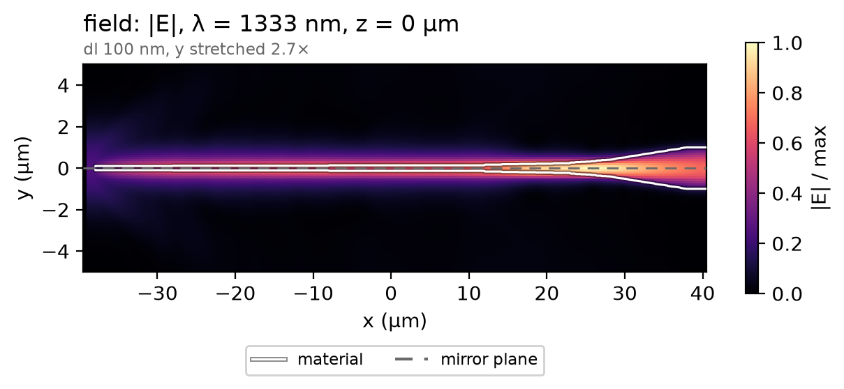
The TE0 field in the plane of the nitride at 1333 nm, the band centre in frequency. The fibre mode enters at the left, the tip picks it up, and the light narrows into the end waveguide as the taper widens; what the tip misses spreads into the cladding and leaves through the PML.

data["TE0"][0].plot_field("field", field="E", z=0.0)
plt.show()

Result

The coupling efficiency is the modal power in the end waveguide over the power the beam launches, read on a plane between the two, so light left in the cladding does not count. The markers are the paper's simulated curves, Fig. 5(a) for TE0 and Fig. 8(a) for TM0, one point in eight plus the peak and the last. The peaks agree in wavelength; ours runs up to 22 percentage points under at the blue end, where the mesh already moves 3 points at 1400 nm and the beam stays 4 µm wide while a fibre's mode grows with wavelength.

# paper-data: bhandari2020_fig5
# Fig. 5(a) TE, 3D BPM; CC BY 4.0, doi:10.1109/JPHOT.2020.3036498; every 8th point, peak, last
# fmt: off
te_nm = [1000.0, 1040.0, 1095.0, 1135.0, 1175.0, 1215.0, 1260.0, 1300.0, 1340.0, 1380.0, 1420.0,
         1460.0, 1465.0, 1500.0, 1540.0, 1580.0, 1620.0, 1660.0, 1700.0, 1740.0, 1780.0, 1820.0,
         1860.0, 1900.0, 1940.0, 1980.0, 1995.0]
te_pct = [52.16, 54.34, 57.78, 61.33, 64.65, 68.67, 75.84, 82.06, 87.43, 91.6, 93.87, 94.6, 94.71,
          94.66, 93.86, 92.14, 89.12, 85.59, 81.27, 76.8, 72.03, 67.04, 62.88, 58.81, 54.7, 50.84,
          49.61]
# fmt: on
paper_te = {"x": te_nm, "y": te_pct, "label": "paper, Fig. 5(a), 3D BPM, TE0"}
# paper-data: bhandari2020_fig8
# Fig. 8(a) TM, 3D BPM; CC BY 4.0, doi:10.1109/JPHOT.2020.3036498; every 8th point, peak, last
# fmt: off
tm_nm = [1005.0, 1045.0, 1085.0, 1125.0, 1165.0, 1205.0, 1245.0, 1285.0, 1325.0, 1365.0, 1405.0,
         1445.0, 1485.0, 1525.0, 1565.0, 1575.0, 1645.0, 1685.0, 1725.0, 1765.0, 1805.0, 1845.0,
         1885.0, 1925.0, 1965.0, 1995.0]
tm_pct = [31.78, 35.8, 39.84, 43.9, 48.02, 52.18, 56.3, 60.44, 64.98, 70.54, 75.74, 80.42, 84.22,
          86.68, 88.14, 88.41, 88.11, 86.81, 85.45, 83.62, 81.1, 77.96, 74.36, 70.12, 65.15, 61.18]
# fmt: on
paper_tm = {"x": tm_nm, "y": tm_pct, "label": "paper, Fig. 8(a), 3D BPM, TM0"}

def spectrum(sim, data):
    """Coupling efficiency (%) against wavelength (nm): guided over launched power."""
    power = sim.port_monitors["out"].mode_power(data, direction="+")
    f = np.array(sorted(power, reverse=True))  # ascending wavelength
    guided = np.array([power[k] for k in f])
    launched_w = np.asarray(data["launched"].values, float).ravel()
    return ph.c0 / f * 1e9, 100 * guided / launched_w


eta = {}
for pol in sims:
    (nm_blue, blue), (nm_red, red) = (spectrum(s, d) for s, d in zip(sims[pol], data[pol]))
    print(f"{pol} at {wlen_split * 1e3:.0f} nm: blue run {blue[-1]:.1f} %, red run {red[0]:.1f} %")
    eta[pol] = np.concatenate([nm_blue, nm_red[1:]]), np.concatenate([blue, red[1:]])
ph.viz.plot_comparison(
    eta["TE0"][0],
    {f"PhotonHub, {pol}": eta[pol] for pol in eta},
    reference=[paper_te, paper_tm],
    ylabel="fibre-to-chip coupling efficiency (%)",
    ylim=(0, 100),
)
plt.show()
at_1550 = {pol: float(np.interp(1550.0, *eta[pol])) for pol in eta}
print(f"TE0 coupling at 1550 nm: {at_1550['TE0']:.1f} % | TM0: {at_1550['TM0']:.1f} %")

output

TE0 at 1400 nm: blue run 88.4 %, red run 88.6 %

output

TM0 at 1400 nm: blue run 77.7 %, red run 77.8 %

output

TE0 coupling at 1550 nm: 87.1 % | TM0: 90.9 %

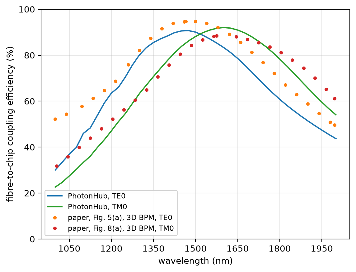
At 100 nm cells TE0 reads 87.1 % at 1550 nm and TM0 90.9 %; at 60 nm cells, 88.2 % and 89.9 %, not shown converged; the paper's 3D beam propagation method, 93.5 % and 87.8 %. At 1400 nm the two runs agree within 0.3 points; the meshes, by about 3. The runs use a uniform mesh, subpixel averaging on, constant indices, 12 PML layers and one mirror plane normal to y.