Optimal 90-degree waveguide bend
A photonic chip routes light in waveguides, narrow strips of silicon that hold light in by total internal reflection, as an optical fibre does. Light travels along a waveguide as a mode, a field pattern that keeps its shape; the simplest, TE0, has its electric field across the strip. Every layout turns its waveguides, and a 90-degree bend joins two guides at right angles. The usual bend is a circular arc, but its curvature jumps from zero to one over the radius at each end: there the straight guide's mode does not fit the bend, and part of the light is lost, more as the bend shrinks. An optimal bend lets its curvature grow smoothly from zero at each end to a peak in the middle, shaped so that it radiates the least for its footprint, the distance the turn takes up. The figure of merit is the loss per bend in decibels (dB), a logarithmic scale on which 0.01 dB is about 0.2 % of the power; bends a few micrometres across lose a few thousandths to a few hundredths of a dB.
This notebook builds the bend of Bahadori, Nikdast, Cheng and Bergman, J. Lightwave Technol. 37, 3044 (2019) on a 400 x 220 nm silicon strip with a 5 µm footprint, beside a circular bend of the same footprint: 0.0017 dB per bend at 1550 nm against the paper's 0.0019 dB, and 0.0117 dB for the circular bend against 0.0125 dB.
Parameters
The design numbers are the paper's; the shape needs only the exponent b of
its bend-loss fit. The band is the paper's C-band. A uniform mesh gives the
circular bend the same cells. The leads, five mode widths, run on through the
PML, the absorbing layers at the walls; the clearances keep five decay lengths
of the mode's tail. TE0 is even about the slab's mid-plane, so a mirror plane
there halves the run. A loss this small needs the field to decay to 1e-9.
# design, the paper's symbols (Sec. II and III)
w = 0.40  # strip width (µm)
h = 0.22  # silicon thickness (µm)
R0 = 5.0  # footprint: the guide axes are R0 apart (µm)
b = 2.49  # exponent of the loss fit a R^-b (Sec. II)
R0_sweep = (3.0, 4.0, 5.0, 8.0)  # footprints of the sweep (µm)
paper_optimal_db = 0.0019  # paper, stated 3D FDTD loss at R0 (dB)
paper_circular_db = 0.0125  # paper, stated circular loss at R0 (dB)
# simulation choices
wlen_min = 1.50  # band start (µm)
wlen_max = 1.60  # band end (µm)
n_wlen = 21  # wavelengths read out
cells_per_wlen = 12  # mesh cells per wavelength in silicon
lead = 2.0  # straight guide before each port (µm)
overshoot = 1.5  # leads drawn on past the ports (µm)
clearance = 0.8  # silicon edge to PML, in plane (µm)
clearance_z = 0.8  # core to PML, above and below (µm)
pml = 12  # PML layers
symmetry = (0, 0, 1)  # mirror plane through the slab centre
shutoff = 1e-9  # field decay that ends the run
dft_shutoff = 0.0  # 0 = no spectrum-settling check
n_path = 40000  # integration steps along the bend
keep = 200  # the outline keeps one step in this many

wlen = np.linspace(wlen_min, wlen_max, n_wlen)  # wavelengths (µm)
wlen0 = 0.5 * (wlen_min + wlen_max)  # band centre (µm)
f0 = ph.c0 / (wlen0 * 1e-6)  # band-centre frequency (Hz)
Geometry
The bend joins a guide along x to one along y whose axes are R0 apart. The
paper's Eq. (15) and (17) set the curvature by the direction of travel θ:
A sin(θ)^(1/b) up to 45 degrees and A cos(θ)^(1/b) after, zero at both ends;
R0 fixes A. Integrating gives the centreline; each point moved half the
width along the normal gives the sidewalls of a ph.Polygon, an outline in
the chip plane extruded through the silicon, and ph.Structure makes it
silicon. The circular bend follows a quarter circle. The sweep redraws both,
so the outline is a function of the kind and the footprint.
def bend(kind, radius):
    theta = np.linspace(0.0, np.pi / 2, n_path + 1)  # direction of travel
    if kind == "circular":
        x, y = radius * np.sin(theta), radius * (1 - np.cos(theta))
    else:
        mid = 0.5 * (theta[1:] + theta[:-1])
        curv = np.where(mid <= np.pi / 4, np.sin(mid), np.cos(mid)) ** (1 / b)  # over A, Eq. (17)
        ds = np.diff(theta) / curv  # path length per step
        x = np.concatenate([[0.0], np.cumsum(np.cos(mid) * ds)])
        y = np.concatenate([[0.0], np.cumsum(np.sin(mid) * ds)])
        x, y = x * radius / x[-1], y * radius / x[-1]  # the scale A that fits the footprint
    x, y, theta = x[::keep], y[::keep], theta[::keep]
    x = np.concatenate([[-lead - overshoot], x, [radius]]) - radius / 2  # a lead in, one out
    y = np.concatenate([[0.0], y, [radius + lead + overshoot]]) - radius / 2
    theta = np.concatenate([[0.0], theta, [np.pi / 2]])
    left = list(zip(x - w / 2 * np.sin(theta), y + w / 2 * np.cos(theta)))
    right = list(zip(x + w / 2 * np.sin(theta), y - w / 2 * np.cos(theta)))
    shape = ph.Polygon(axis="z", vertices_um=right + left[::-1], slab_bounds_um=(-h / 2, h / 2))
    return [ph.Structure(geometry=shape, medium=ph.materials.Si)]
Simulation
A ph.Port is a plane across a guide: its centre, the axis the light travels
along, and the guide's width and thickness. The simulation solves the TE0 mode
there, launches it at in on the x guide and reads the modal power at out
on the y guide. The SDK sizes the window the mode is read in so the mode is
30 dB down at its edge, with a 20 % margin.
ports = [
    ph.Port("in", (-lead - R0 / 2, -R0 / 2, 0.0), "x", w, thickness_um=h),
    ph.Port("out", (R0 / 2, R0 / 2 + lead, 0.0), "y", w, thickness_um=h),
]
ph.Simulation holds the setup. ph.Domain fits the box around the bend and
continues each guide through the PML; ph.Mesh sets cells_per_wlen cells
per wavelength in the silicon, uniform here, with subpixel averaging at the
interfaces. The field monitor records the chip plane at the band centre.
field = ph.ProfileMonitor.plane(
    "field",
    "z",
    0.0,
    wlens_um=wlen0,
    fields=("Ex", "Ey", "Ez", "Hz"),  # Hz follows the light round the turn
)
sim = ph.Simulation(
    domain=ph.Domain(clearance_um=(clearance, clearance, clearance_z)),
    mesh=ph.Mesh(cells_per_wlen=cells_per_wlen, uniform=True),
    background=ph.materials.SiO2,  # oxide cladding
    pml_num_layers=pml,
    structures=bend("optimal", R0),
    symmetry=symmetry,
    wlens_um=wlen,  # wavelengths read out at the ports
    ports=ports,
    source="in",  # the port that launches TE0
    run=ph.RunSpec(shutoff=shutoff, dft_shutoff=dft_shutoff),
    monitors=[field],
)
sim.plot_index(z=0.0)
plt.show()
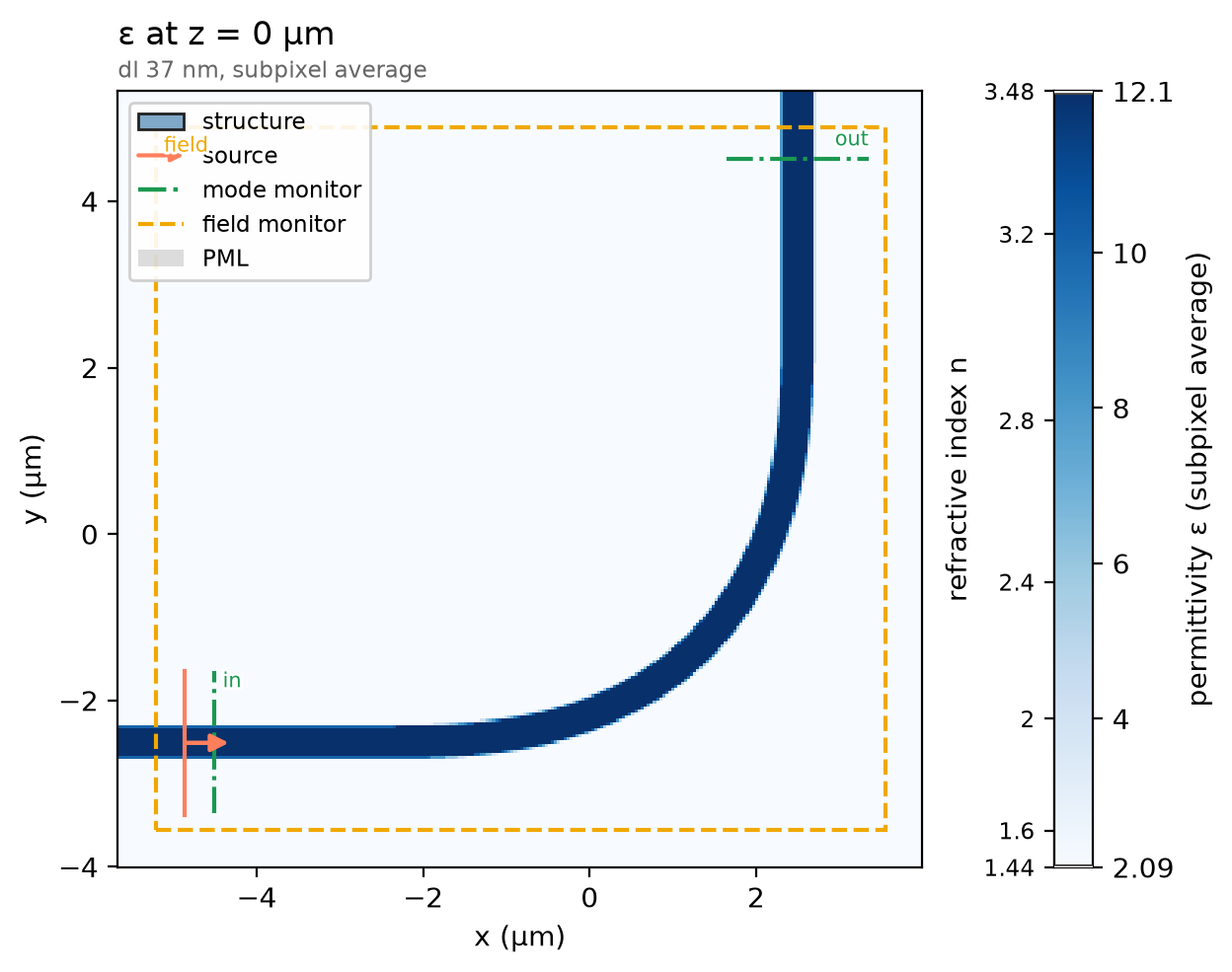
ph.run_local runs the solver on this computer; ph.cloud.run_quoted runs it
on a cloud GPU.
data = ph.run_local(sim, quiet=True)
# On a cloud GPU instead, with GPU and SOLVER from your closed-test guide:
# data = ph.cloud.run_quoted(sim, device=GPU, solver=SOLVER)
Field
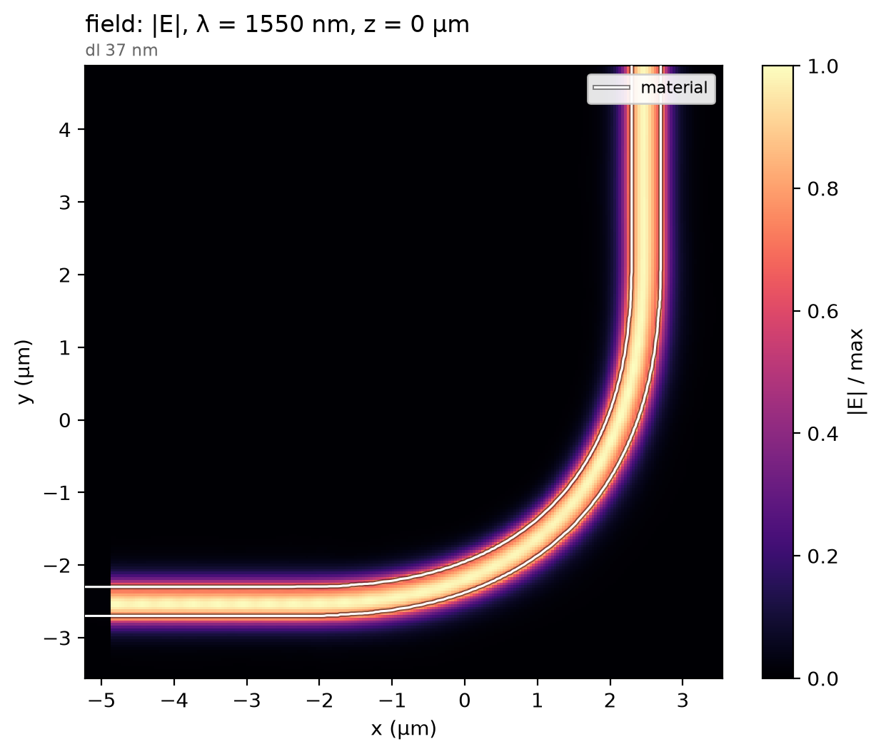
The mode follows the bend with no step at either end: the curvature starts at zero, so the straight guide's mode is already the local bend mode where they meet.
Result
The loss is −10 log₁₀ of the TE0 modal power at the output over the launched power, as the paper reports its 3D FDTD result. The circular bend of the same footprint runs on the same mesh. The dashed lines are the paper's stated values; its licence does not allow re-plotting its curves.
loss_db = -10 * np.log10(data.transmission("out"))  # optimal bend (dB)
circular = ph.run_local(sim.with_changes(structures=bend("circular", R0)), quiet=True)
loss_circular_db = -10 * np.log10(circular.transmission("out"))  # circular bend (dB)
ph.viz.plot_comparison(
    loss_db.wlen_um * 1e3,
    {"optimal bend": loss_db, "circular bend": loss_circular_db},
    stated=[
        (paper_optimal_db, "paper, stated (3D FDTD, optimal)"),
        (paper_circular_db, "paper, stated (3D FDTD, circular)"),
    ],
    ylabel="loss per 90-degree bend (dB)",
    ylim=(0, 0.025),
)
plt.show()
opt = float(loss_db.sel(f=f0, method="nearest"))
circ = float(loss_circular_db.sel(f=f0, method="nearest"))
print(f"optimal bend {opt:.4f} dB | circular bend {circ:.4f} dB | reduction {1 - opt / circ:.0%}")
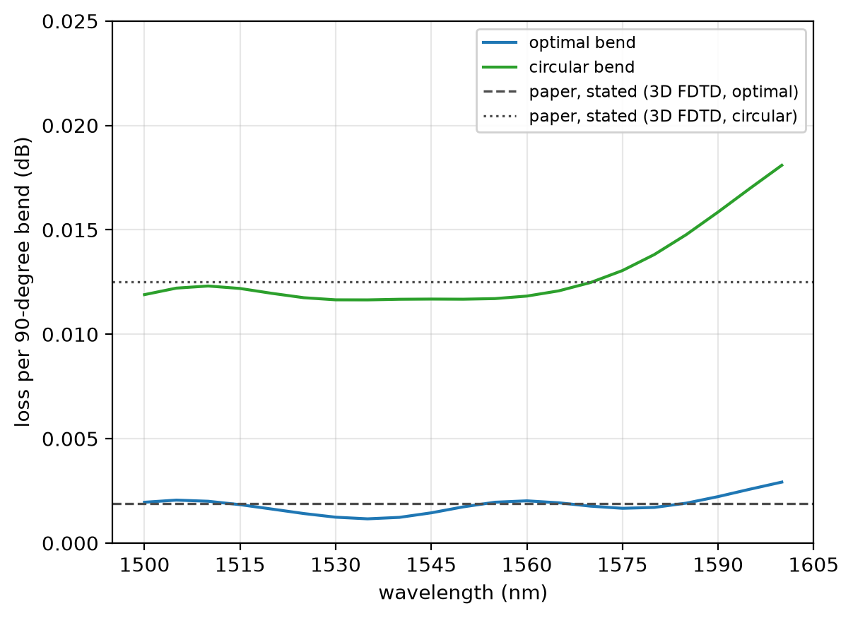
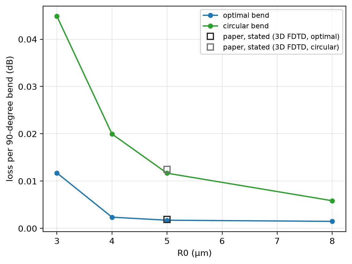
At 12 cells per wavelength the optimal bend's loss reads 0.0017 dB at 1550 nm; converged, 0.0008 dB; the paper's 3D FDTD, 0.0019 dB. The circular bend reads 0.0117 dB; converged, 0.0118 dB; the paper's, 0.0125 dB. Both converged values subtract a straight guide read on the same mesh. The runs use a uniform mesh, subpixel averaging on, non-dispersive silicon and oxide, 12 PML layers and one mirror plane through the slab.
Sweep
The footprint is the knob. Each point is a full run of both bends at one
R0, with the ports moved to its guides. At 8 µm the optimal bend reads
little below 5 µm: at this mesh numerical scattering at the stepped sidewalls
holds both up, so each is an upper bound. The squares are the paper's stated
values at 5 µm.
loss_opt, loss_circ = [], []
for radius in R0_sweep:
    at_in = (-lead - radius / 2, -radius / 2, 0.0)  # the ports move with the guides
    at_out = (radius / 2, radius / 2 + lead, 0.0)
    moved = [
        ph.Port("in", at_in, "x", w, thickness_um=h),
        ph.Port("out", at_out, "y", w, thickness_um=h),
    ]
    for kind, loss in (("circular", loss_circ), ("optimal", loss_opt)):
        out = ph.run_local(sim.with_changes(structures=bend(kind, radius), ports=moved), quiet=True)
        loss.append(-10 * np.log10(float(out.transmission("out").sel(f=f0, method="nearest"))))
ph.viz.plot_comparison(
    np.array(R0_sweep),
    {"optimal bend": np.array(loss_opt), "circular bend": np.array(loss_circ)},
    stated=[
        (R0, paper_optimal_db, "paper, stated (3D FDTD, optimal)"),
        (R0, paper_circular_db, "paper, stated (3D FDTD, circular)"),
    ],
    xlabel="R0 (µm)",
    ylabel="loss per 90-degree bend (dB)",
)
plt.show()
pairs = zip(R0_sweep, loss_opt, loss_circ)
print(" | ".join(f"R0 {r:.0f}: {o:.4f} vs {c:.4f} dB" for r, o, c in pairs))