Ultralow-loss waveguide crossing

A photonic chip carries light in waveguides: narrow strips of silicon that hold light in by total internal reflection, as an optical fibre does. Light travels along a waveguide as a mode, a field pattern that keeps its shape; the simplest, called TE0, has its electric field across the strip. All the waveguides of a chip lie in one silicon layer, so wherever two light paths must cross, their strips have to intersect. At a plain intersection the mode loses the side walls that hold it, spreads out, and part of it scatters out of the chip or into the crossing waveguide. A good crossing widens each arm into a taper before the junction: the mode expands slowly, crosses the gap as a nearly flat wave and narrows again into the far arm. Two numbers rate it, both in decibels (dB), a logarithmic scale on which 0.1 dB is about 2 % of the power. The insertion loss is the power that fails to reach the far arm; good designs lose a few hundredths of a dB. The crosstalk is the power that leaks into the side arms, typically below −40 dB, one part in ten thousand.

This notebook builds the crossing of Ma et al., Opt. Express 21, 29374 (2013) from the paper's Table 1 and reads its TE0 insertion loss across 1500 to 1600 nm: 0.0177 dB at 1550 nm, against the paper's stated 3D FDTD value of 0.017 dB. The crosstalk is −65 dB.

Parameters

The design numbers are the paper's Table 1; the spline's end condition is assumed. The band is the paper's, the mesh its 14 cells per wavelength; the leads are two mode widths and the clearances three decay lengths of the mode tail. A mirror plane on the input axis halves the run.

import matplotlib.pyplot as plt
import numpy as np
from scipy.interpolate import CubicSpline

import photonhub as ph

# design, the paper's Table 1
w = 0.50  # routing waveguide width (µm)
h = 0.22  # silicon thickness (µm)
L = 4.5  # taper length, end to crossing centre (µm)
w_knots = [0.5, 0.6, 0.95, 1.32, 1.44, 1.46, 1.466, 1.52, 1.58, 1.62, 1.76, 2.15, 0.5]  # (µm)
spline = "natural"  # assumed spline end condition
paper_il_db = 0.017  # paper, stated 3D FDTD loss at 1550 nm (dB)

# simulation choices
wlen_min = 1.50  # band start (µm)
wlen_max = 1.60  # band end (µm)
n_wlen = 21  # wavelengths read out
cells_per_wlen = 14  # mesh cells per wavelength in silicon
lead = 1.0  # straight guide before each port (µm)
clearance = 0.6  # silicon edge to PML, in plane (µm)
clearance_z = 0.8  # core to PML, above and below (µm)
pml = 12  # PML layers
symmetry = (0, -1, 0)  # mirror normal to y; (0, 0, 0) if asymmetric
shutoff = 1e-7  # field decay that ends the run
dft_shutoff = 0.0  # 0 = no spectrum-settling check

wlen = np.linspace(wlen_min, wlen_max, n_wlen)  # wavelengths (µm)
wlen0 = 0.5 * (wlen_min + wlen_max)  # band centre (µm)
f0 = ph.c0 / (wlen0 * 1e-6)  # band-centre frequency (Hz)

Geometry

The crossing is four identical tapers. Each is a ph.Polygon: an outline in the chip plane (vertices_um, counter-clockwise) extruded through the silicon (slab_bounds_um), its half-width a spline through the paper's thirteen knots. The x- taper is drawn once and turned to the other arms.

s = np.linspace(0.0, L, 121)  # along a taper, end to centre (µm)
knots = np.linspace(0.0, L, len(w_knots))  # knot positions (µm)
half = CubicSpline(knots, w_knots, bc_type=spline)(s) / 2  # half-width (µm)
edge = [(si - L, hi) for si, hi in zip(s, half)]  # upper sidewall of the x- taper
outline = [(u, -v) for u, v in edge] + edge[::-1]  # counter-clockwise outline
arms = [
    outline,  # x- arm
    [(-u, -v) for u, v in outline],  # x+ arm, half a turn
    [(-v, u) for u, v in outline],  # y- arm, a quarter turn
    [(v, -u) for u, v in outline],  # y+ arm, three quarter turns
]
tapers = [ph.Polygon(axis="z", vertices_um=p, slab_bounds_um=(-h / 2, h / 2)) for p in arms]

A straight ph.Box lead joins each taper to its port. ph.Structure gives every shape a medium, here the library's silicon.

leads = [
    ph.Box(center_um=(-(L + lead / 2), 0.0, 0.0), size_um=(lead, w, h)),  # x- lead
    ph.Box(center_um=(L + lead / 2, 0.0, 0.0), size_um=(lead, w, h)),  # x+ lead
    ph.Box(center_um=(0.0, -(L + lead / 2), 0.0), size_um=(w, lead, h)),  # y- lead
    ph.Box(center_um=(0.0, L + lead / 2, 0.0), size_um=(w, lead, h)),  # y+ lead
]
structures = [ph.Structure(geometry=g, medium=ph.materials.Si) for g in tapers + leads]

Simulation

A ph.Port is a plane across a guide: its centre, the axis the light travels along, and the guide's width and thickness. The simulation solves the TE0 mode there, launches it from the source port and reads the modal power at every port. x- is the input, x+ the through port, y- and y+ the side arms. The SDK sizes the window each mode is read in so the mode is 30 dB down at its edge, with a 20 % margin.

arm = L + lead  # centre to each port plane (µm)
ports = [
    ph.Port("x-", (-arm, 0.0, 0.0), "x", w, thickness_um=h),  # input
    ph.Port("x+", (arm, 0.0, 0.0), "x", w, thickness_um=h),  # through
    ph.Port("y-", (0.0, -arm, 0.0), "y", w, thickness_um=h),  # side arm
    ph.Port("y+", (0.0, arm, 0.0), "y", w, thickness_um=h),  # side arm
]

ph.Simulation holds the setup. ph.Domain fits the box around the structures and continues each guide through the PML. ph.Mesh grades the mesh: cells_per_wlen cells per wavelength in the silicon, coarser in the oxide, with subpixel averaging at the interfaces. The field monitor records the chip plane; the auto-shutoff ends the run once the light has left.

field = ph.ProfileMonitor(
    name="field",  # the chip plane, at the band centre
    center_um=(0.0, 0.0, 0.0),
    size_um=(2 * L, 2 * L, 0.0),
    fields=("Ex", "Ey", "Ez"),
    freqs_hz=(f0,),
)
sim = ph.Simulation(
    domain=ph.Domain(clearance_um=(clearance, clearance, clearance_z)),
    mesh=ph.Mesh(cells_per_wlen=cells_per_wlen),
    background=ph.materials.SiO2,  # oxide cladding
    pml_num_layers=pml,
    structures=structures,
    symmetry=symmetry,
    wlens_um=wlen,  # wavelengths read out at the ports
    ports=ports,
    source="x-",  # the port that launches TE0
    run=ph.RunSpec(shutoff=shutoff, dft_shutoff=dft_shutoff),
    monitors=(field,),
)
sim.plot_index(z=0.0)
plt.show()

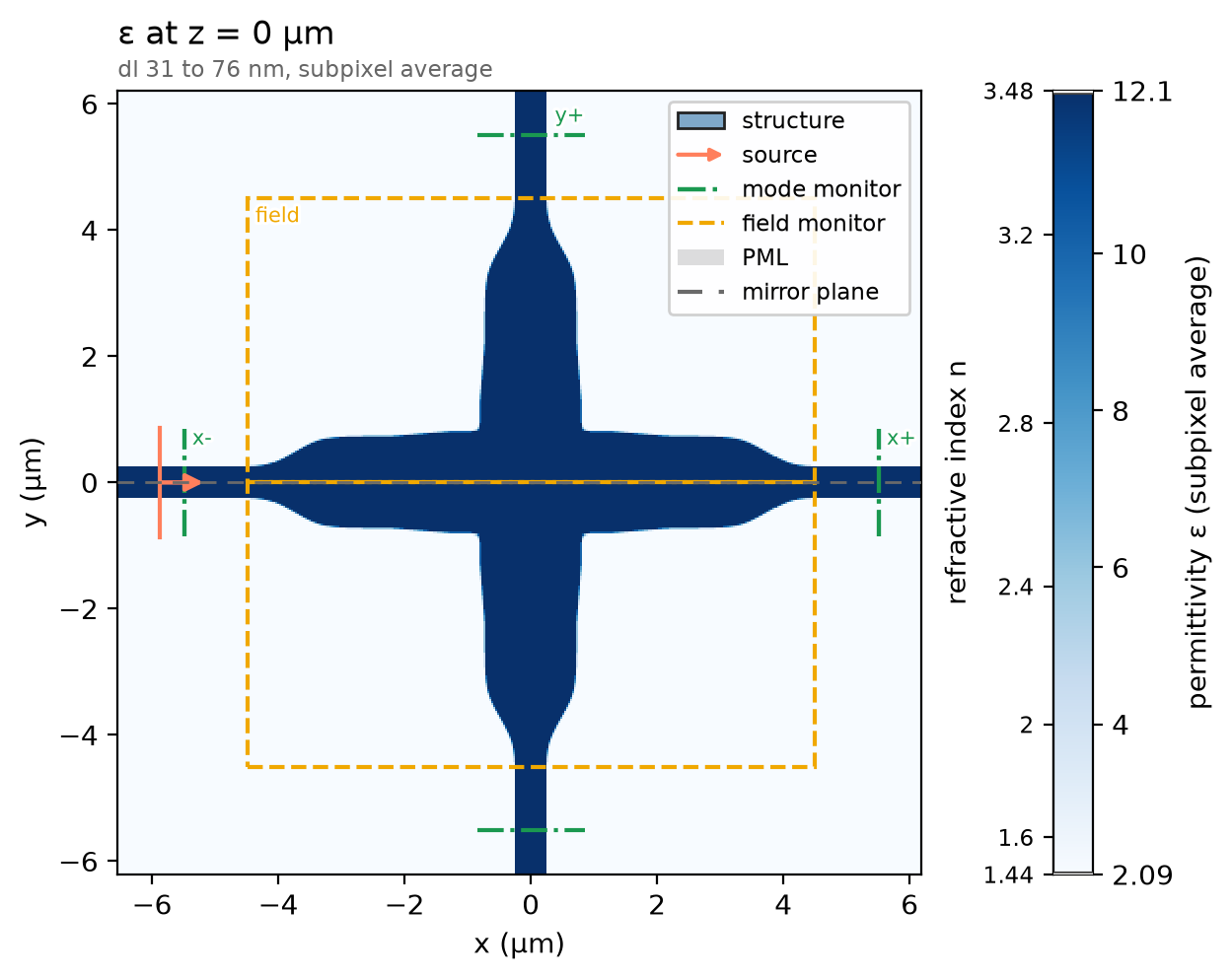
ph.run_local runs the solver on this computer; ph.cloud.run_quoted runs it on a cloud GPU.

data = ph.run_local(sim, quiet=True)
# On a cloud GPU instead, with GPU and SOLVER from your closed-test guide:
# data = ph.cloud.run_quoted(sim, device=GPU, solver=SOLVER)

Field

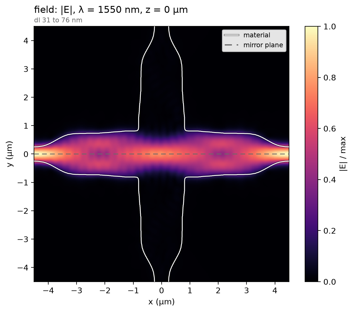
The mode widens along the input taper, crosses the junction as a nearly flat front and refocuses into the far arm, so almost nothing reaches the side arms. The half below the mirror plane is the image of the half that ran.

data.plot_field("field", field="E", z=0.0, freq=f0)
plt.show()

Result

The insertion loss is −10 log₁₀ of the through port's modal power over the launched modal power. The dashed line is the paper's stated value at 1550 nm; the article's licence does not allow re-plotting its curve here.

T = data.transmission("x+")  # through-port modal power ratio
il_db = -10 * np.log10(T)  # insertion loss (dB)
xt_db = 10 * np.log10(float(data.transmission("y+").sel(f=f0, method="nearest")))
ph.viz.plot_comparison(
    il_db,
    stated=(paper_il_db, "paper, stated (loss at 1550 nm)"),
    ylabel="insertion loss (dB)",
    ylim=(0, 0.1),
)
plt.show()
il_1550 = float(il_db.sel(f=f0, method="nearest"))
print(f"insertion loss at 1550 nm: {il_1550:.4f} dB | TE0 crosstalk {xt_db:.0f} dB")

output

insertion loss at 1550 nm: 0.0177 dB | TE0 crosstalk -65 dB

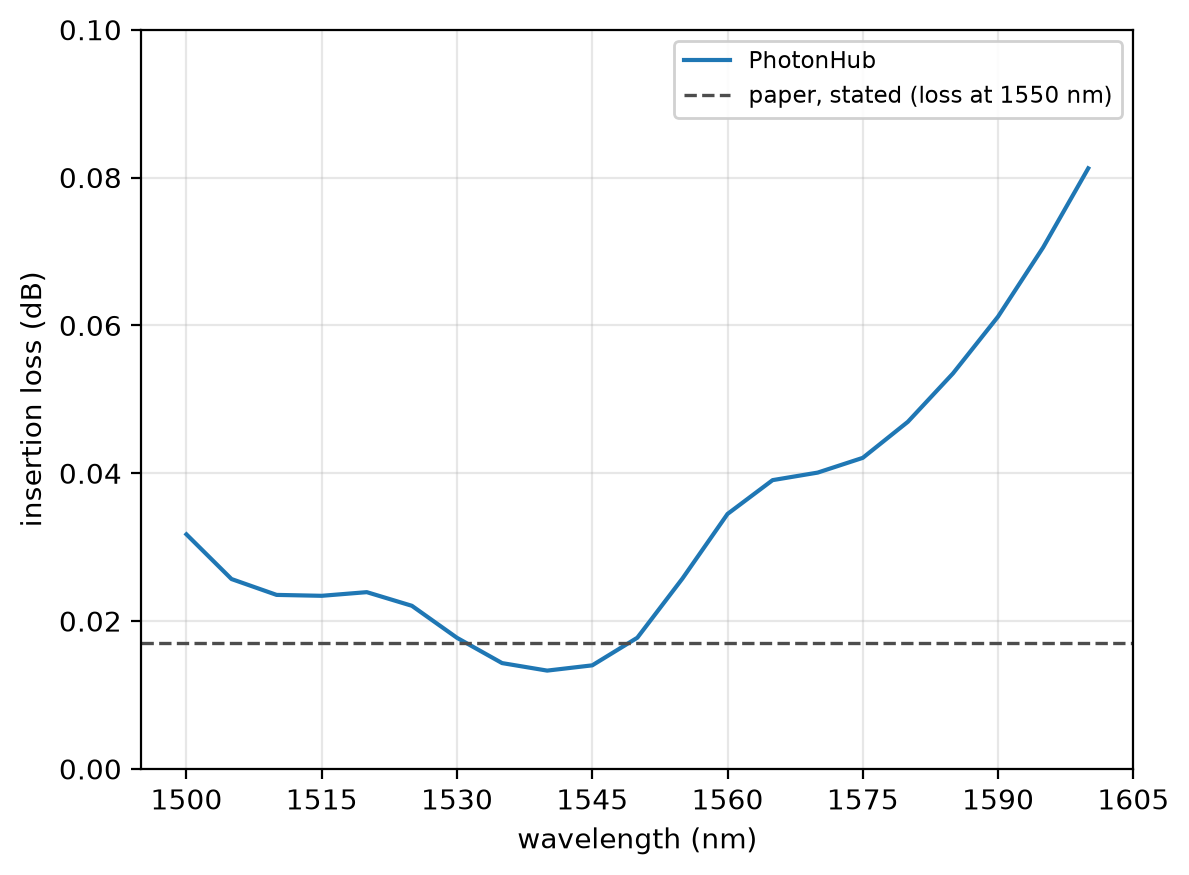
At 14 cells per wavelength the insertion loss reads 0.0177 dB at 1550 nm; converged, 0.0145 dB; the paper's 3D FDTD, 0.017 dB. The run uses a graded mesh of 14 cells per wavelength in the silicon, subpixel averaging on, non-dispersive silicon and oxide, 12 PML layers and one mirror plane normal to y.