Y-junction with a chosen splitting ratio
A photonic chip routes light in waveguides, narrow strips of silicon that hold light in by total internal reflection, as an optical fibre does. Light travels along a waveguide as a mode, a field pattern that keeps its shape; the simplest, TE0, has its electric field across the strip. Many circuits must divide that light between two waveguides, to tap a little for a monitor or to weight the branches of a filter. A Y-junction widens the guide and splits it into two arms. A symmetric one splits evenly; shifting or narrowing an arm to make it uneven tends to scatter light or to make the ratio drift with wavelength. Here the widened region is bounded on each side by S-curves of circular arcs; a smaller radius on one side steers more of the mode into the other arm, so one number sets the ratio. Two figures rate it, in decibels (dB), a logarithmic scale on which 3 dB is a factor of two: the splitting ratio, one arm's power over the other's, and the excess loss, the power reaching neither arm, typically a few tenths of a dB.
This notebook builds the junction of Lin and Shi, Opt. Express 27, 14338 (2019) and reads both arms across 1500 to 1600 nm. At the symmetric setting each arm carries 0.483 of the input and the arms differ by 0.0006 dB at 1550 nm, against the paper's stated 0.48 and 0 dB. A sweep of the one radius follows.
Parameters
The design numbers are the paper's Fig. 1 and its stated results. The outputs sit 0.20 µm apart and stay coupled, so bends added for the simulation separate the arms before the ports. The band brackets the paper's 1535 to 1580 nm. A uniform mesh gives every radius of the sweep the same cells. The leads are two mode widths; the clearances keep three decay lengths of the mode's tail ahead of the PML, the absorbing layers at the walls.
# design, the paper's symbols (Fig. 1)
w0 = 0.50  # input and output guide width (µm)
h = 0.22  # silicon thickness (µm)
L = 2.32  # length of the splitting region (µm)
w = 0.70  # half-width of the splitting region (µm)
D = 0.20  # gap between the output branches (µm)
R1 = 1.70  # lower boundary, first radius (µm)
R2 = 1.00  # lower boundary, second radius (µm)
r1 = 1.70  # upper first radius, the knob (µm); R1: even
r1_sweep = (1.70, 1.32, 0.92, 0.72, 0.42, 0.22)  # (µm)
paper_T_arm = 0.48  # paper, Sec. 4: each arm at r1 = R1
paper_r1 = (0.22, 0.92, 1.70)  # paper, Sec. 4: radii (µm)
paper_ratio_db = (-12.6, -5.5, 0.0)  # paper, Sec. 4: ratio there (dB)
# simulation choices
wlen_min = 1.50  # band start (µm)
wlen_max = 1.60  # band end (µm)
n_wlen = 21  # wavelengths read out
cells_per_wlen = 12  # mesh cells per wavelength in silicon
fanout = 3.0  # added: length of the access bends (µm)
offset_out = 1.0  # added: arm centres at the ports (µm)
lead = 1.0  # straight guide before each port (µm)
clearance = 0.8  # silicon edge to PML, in plane (µm)
clearance_z = 0.8  # core to PML, above and below (µm)
pml = 12  # PML layers
shutoff = 1e-7  # field decay that ends the run
dft_shutoff = 0.0  # 0 = no spectrum-settling check
n_arc = 70  # outline points along each arc and bend

wlen = np.linspace(wlen_min, wlen_max, n_wlen)  # wavelengths (µm)
wlen0 = 0.5 * (wlen_min + wlen_max)  # band centre (µm)
f0 = ph.c0 / (wlen0 * 1e-6)  # band-centre frequency (Hz)
Geometry
The splitting region follows the paper's Fig. 1. On each side its outer edge
is an S-curve out to the half-width w, a straight section, and an S-curve
back to the outer edge of an output guide; each S is two equal tangent arcs,
drawn by s_curve.
a = (w - w0 / 2) / 4  # paper Eq. (2)
b = (w - w0 - D / 2) / 2  # paper Eq. (2)
half_L = L / 2  # the region runs from -L/2 to L/2 (µm)
y_in = w0 / 2  # the region's outer edge at the input (µm)
y_out = w0 + D / 2  # the region's outer edge at the output (µm)
arm = half_L + fanout + lead  # centre to each port plane (µm)


# an S-bend of two equal tangent arcs from (0, 0), heading +x, to dy across
def s_curve(radius, dy):
    phi = np.arccos(1 - abs(dy) / (2 * radius))  # the angle of each arc
    sign = 1 if dy >= 0 else -1
    first = [(radius * np.sin(t), radius * (1 - np.cos(t))) for t in np.linspace(0, phi, n_arc)]
    x1, y1 = first[-1]
    cx, cy = x1 + radius * np.sin(phi), y1 - radius * np.cos(phi)  # the second arc's centre
    ts = np.linspace(phi * (n_arc - 1) / n_arc, 0, n_arc)
    second = [(cx - radius * np.sin(t), cy + radius * np.cos(t)) for t in ts]
    return [(px, sign * py) for px, py in first + second]
The lower side keeps the published radii; the upper side's second radius and
straight section follow from r1 by the paper's Eq. (2) and (3). A gap on the
axis opens into the branches. Each half is a ph.Polygon, an outline in the
chip plane (vertices_um) extruded through the silicon (slab_bounds_um),
drawn by a function of the radius that the sweep calls again.
def region(radius):
    rho = (radius - a) / (R1 - a) * (R2 - b) + b  # upper second radius, Eq. (2)
    lift = R2 * np.sqrt(1 - ((R2 - b) / R2) ** 2) - rho * np.sqrt(1 - ((rho - b) / rho) ** 2)
    x_tip = half_L - 0.5 * s_curve(rho, w - y_out)[-1][0]  # the branch point on the axis
    halves = []
    for s, r_a, r_b, straight in ((1, radius, rho, max(0.0, lift)), (-1, R1, R2, 0.0)):
        first = s_curve(r_a, s * (w - y_in))  # out to the half-width w
        second = s_curve(r_b, -s * (w - y_out))  # back to the output guide
        x = -half_L + (L - (first[-1][0] + straight + second[-1][0]))  # after the input lead
        pts = [(-half_L, s * y_in), (x, s * y_in)]
        pts += [(x + px, s * y_in + py) for px, py in first]
        x += first[-1][0]
        pts += [(x + straight, s * w)]  # the straight section, Eq. (3)
        x += straight
        pts += [(x + px, s * w + py) for px, py in second]
        pts += [(half_L, s * y_out)]
        outer = pts[:1]
        for p in pts[1:]:  # drop repeated points
            if np.hypot(p[0] - outer[-1][0], p[1] - outer[-1][1]) > 1e-12:
                outer.append(p)
        gap = [(half_L, s * D / 2), (x_tip, 0.0), (-half_L, 0.0)]  # the branch gap
        vertices = outer + gap
        halves.append(ph.Polygon(axis="z", vertices_um=vertices, slab_bounds_um=(-h / 2, h / 2)))
    return halves
Each output guide leaves the region through a raised-cosine bend and runs
straight to its port; its outline is the centreline moved half a width along
the local normal on either side. The input guide is a ph.Box. ph.Structure
gives every shape a medium, here the library's silicon.
guides = []
for s in (1, -1):  # the top arm, then the bottom arm
    y0 = s * (w0 + D) / 2  # the arm's centre as it leaves the region (µm)
    path = [
        (half_L + fanout * t, y0 + (s * offset_out - y0) * 0.5 * (1 - np.cos(np.pi * t)))
        for t in np.linspace(0, 1, n_arc)
    ]
    path += [(arm, s * offset_out)]  # straight on to the port plane
    left, right = [], []
    for i, (px, py) in enumerate(path):
        (xa, ya), (xb, yb) = path[max(i - 1, 0)], path[min(i + 1, len(path) - 1)]
        dx, dy = xb - xa, yb - ya
        norm = np.hypot(dx, dy)
        left.append((px - w0 / 2 * dy / norm, py + w0 / 2 * dx / norm))
        right.append((px + w0 / 2 * dy / norm, py - w0 / 2 * dx / norm))
    outline = left + right[::-1]
    guides.append(ph.Polygon(axis="z", vertices_um=outline, slab_bounds_um=(-h / 2, h / 2)))
guides.append(ph.Box(center_um=(-(arm + half_L) / 2, 0.0, 0.0), size_um=(arm - half_L, w0, h)))
structures = [ph.Structure(geometry=g, medium=ph.materials.Si) for g in region(r1) + guides]
Simulation
A ph.Port is a plane across a guide: its centre, the axis the light travels
along, and the guide's width and thickness. The simulation solves the TE0 mode
there, launches it at in and reads the modal power at both arms, the same
ports for every radius. The SDK sizes the window the mode is read in so the
mode is 30 dB down at its edge, with a 20 % margin.
ports = [
    ph.Port("in", (-arm, 0.0, 0.0), "x", w0, thickness_um=h),  # input
    ph.Port("o_top", (arm, offset_out, 0.0), "x", w0, thickness_um=h),  # top arm
    ph.Port("o_bot", (arm, -offset_out, 0.0), "x", w0, thickness_um=h),  # bottom
]
ph.Simulation holds the setup. ph.Domain fits the box around the
structures and continues each guide through the PML. ph.Mesh sets
cells_per_wlen cells per wavelength in the silicon, uniform here, with
subpixel averaging at the interfaces. The field monitor records the chip
plane at the band centre.
field = ph.ProfileMonitor.plane("field", "z", 0.0, wlens_um=wlen0)  # the chip plane
sim = ph.Simulation(
    domain=ph.Domain(clearance_um=(clearance, clearance, clearance_z)),
    mesh=ph.Mesh(cells_per_wlen=cells_per_wlen, uniform=True),
    background=ph.materials.SiO2,  # oxide cladding
    pml_num_layers=pml,
    structures=structures,
    wlens_um=wlen,  # wavelengths read out at the ports
    ports=ports,
    source="in",  # the port that launches TE0
    run=ph.RunSpec(shutoff=shutoff, dft_shutoff=dft_shutoff),
    monitors=[field],
)
sim.plot_index(z=0.0)
plt.show()
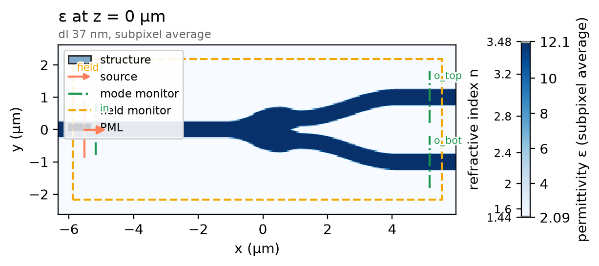
ph.run_local runs the solver on this computer; ph.cloud.run_quoted runs it
on a cloud GPU.
data = ph.run_local(sim, quiet=True)
# On a cloud GPU instead, with GPU and SOLVER from your closed-test guide:
# data = ph.cloud.run_quoted(sim, device=GPU, solver=SOLVER)
Field
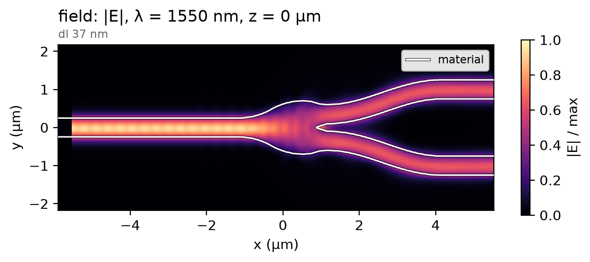
The mode widens into the splitting region, reaches the branch point as one lobe per arm and leaves along the two bends. The change is gradual, so little light radiates at the tip.
Result
Each arm's transmission is its modal power over the launched power; the two curves overlap. The dashed line is the paper's stated value; its licence does not allow re-plotting its curves.
T_top = data.transmission("o_top")  # top arm, modal power ratio
T_bot = data.transmission("o_bot")  # bottom arm, modal power ratio
ph.viz.plot_comparison(
    T_top.wlen_um * 1e3,
    {"top arm": T_top, "bottom arm": T_bot},
    stated=(paper_T_arm, "paper, stated (each arm at r1 = R1)"),
    ylabel="transmission per arm",
    ylim=(0.44, 0.52),
)
plt.show()
top = float(T_top.sel(f=f0, method="nearest"))
bot = float(T_bot.sel(f=f0, method="nearest"))
ratio_db = 10 * np.log10(top / bot)  # splitting ratio, top over bottom (dB)
loss_db = -10 * np.log10(top + bot)  # excess loss (dB)
print(f"top {top:.4f} | bottom {bot:.4f} | ratio {ratio_db:+.4f} dB | loss {loss_db:.3f} dB")
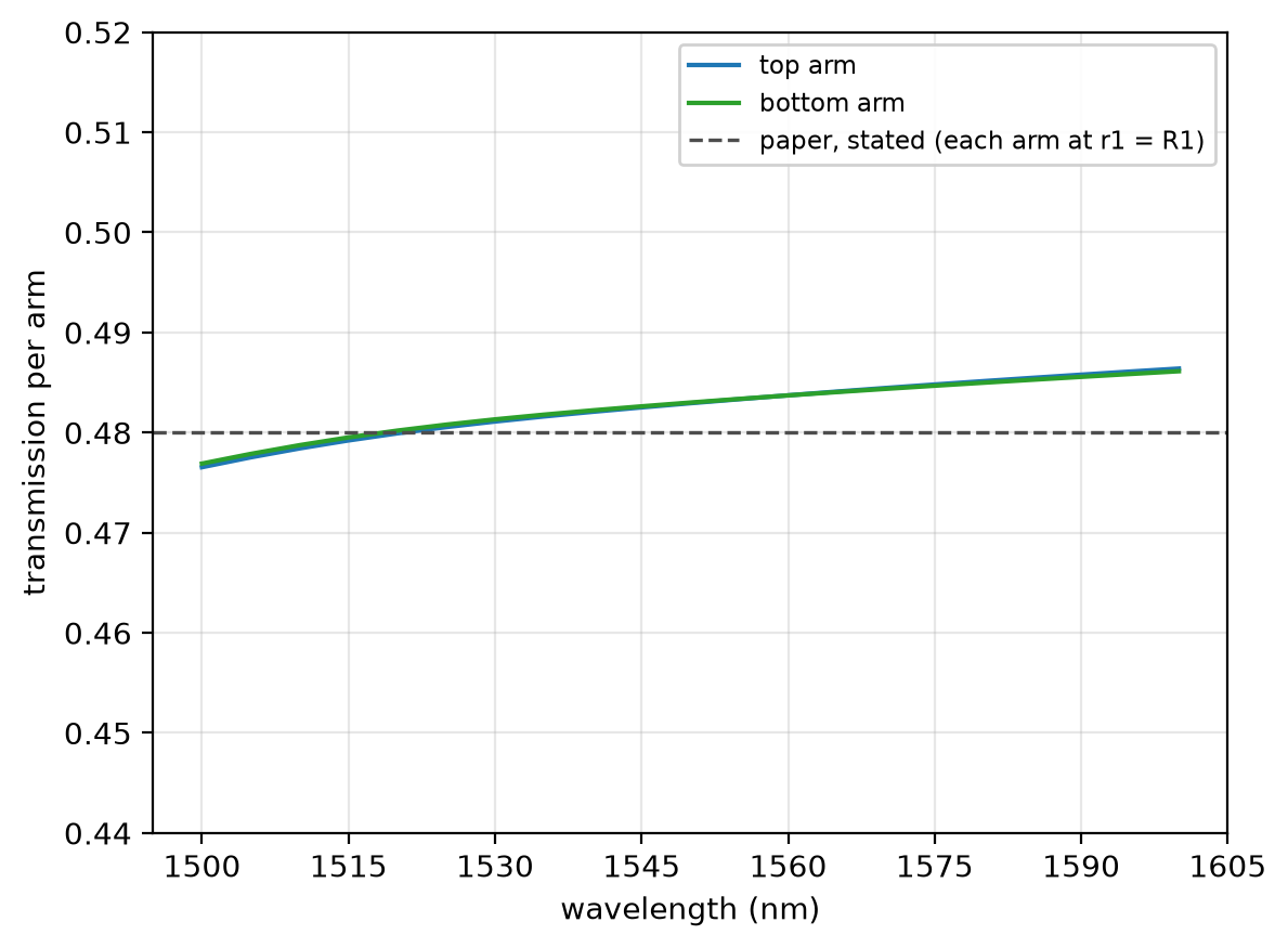
At 12 cells per wavelength each arm carries 0.483 of the input at 1550 nm; at 20 cells, 0.482, not shown converged; the paper's stated value, 0.48. The run uses a uniform mesh of 12 cells per wavelength in the silicon, subpixel averaging on, non-dispersive silicon and oxide, 12 PML layers and no symmetry plane.
Sweep
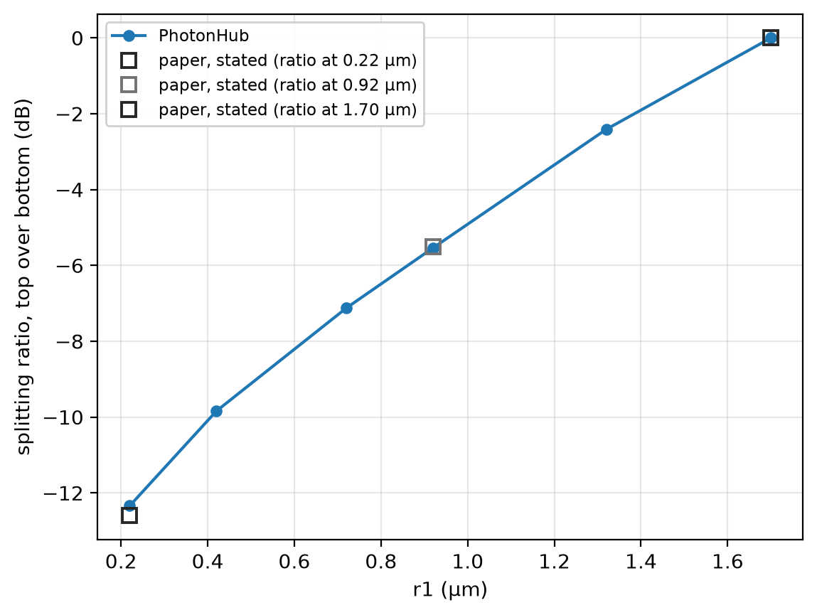
Lowering r1 bends the upper boundary away and moves the branch point off
the axis, so more light turns into the bottom arm. Each point is a full run on
the same mesh; the squares are ratios the paper states for its Fig. 3(a).
sweep_db = []
for radius in r1_sweep:
    shapes = region(radius) + guides
    structures_r = [ph.Structure(geometry=g, medium=ph.materials.Si) for g in shapes]
    out = ph.run_local(sim.with_changes(structures=structures_r), quiet=True)
    top = float(out.transmission("o_top").sel(f=f0, method="nearest"))
    bot = float(out.transmission("o_bot").sel(f=f0, method="nearest"))
    sweep_db.append(10 * np.log10(top / bot))
ph.viz.plot_comparison(
    np.array(r1_sweep),
    np.array(sweep_db),
    stated=[
        (r, v, f"paper, stated (ratio at {r:.2f} µm)") for r, v in zip(paper_r1, paper_ratio_db)
    ],
    xlabel="r1 (µm)",
    ylabel="splitting ratio, top over bottom (dB)",
)
plt.show()
print(" | ".join(f"r1 {r:.2f}: {v:+.1f} dB" for r, v in zip(r1_sweep, sweep_db)))