Curved directional coupler

Two curved silicon waveguides share light where they run close together. This example follows a TE₀ input through the device and compares the power at its bar and cross outputs with Chen et al. (2017), Fig. 4a. The field and spectra below use the completed 12.5 nm simulation.

Electric-field magnitude at 1565 nm. Brightness is normalized for display, not transmission. Oxide cladding is hidden to show the silicon guides.

Set up the coupler

The two guides follow circular arcs joined to straight sections. Launch the TE₀ mode in the upper guide; the bar monitor follows that guide and the cross monitor measures power transferred to the lower guide.

Parameter	Value
Guide widths / height	0.4 µm / 0.25 µm
Gap	0.2 µm
Bend center radius / curved length	26 µm / 8.1 µm
Each tangent straight section	1.8 µm
Refractive indices	Silicon 3.48, oxide 1.444
Mesh	12.5 nm; contour subpixel averaging
Boundary	TE symmetry at z = 0; 0.6 µm PML, 48 layers
Source / output band	TE₀ at 1565 nm / 1520–1620 nm, 21 wavelengths
Simulation duration	2.000021 ps, 83,921 time steps

The model uses lossless constant indices, vertical sidewalls and homogeneous oxide; finite buried-oxide and cladding interfaces are omitted.

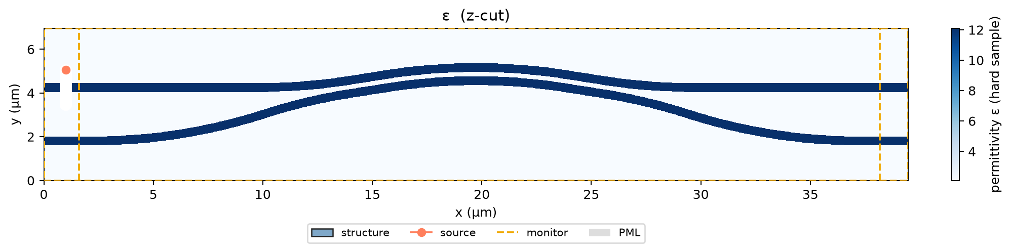
The recorded GPU run took 16.1 minutes to prepare and 12.5 minutes to propagate.

Field profile

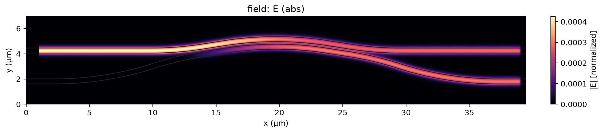
Saved electric-field magnitude |E| at 1565 nm in the horizontal x-y monitor plane, from the full 12.5 nm simulation. Color shows field magnitude, not transmission efficiency.

Compare the two outputs

Normalize each output by the total power in both guides: q_bar = T_bar / (T_bar + T_cross) and q_cross = T_cross / (T_bar + T_cross). These fractions describe the power split; they are not insertion loss.

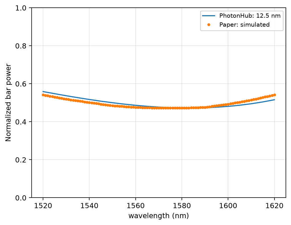
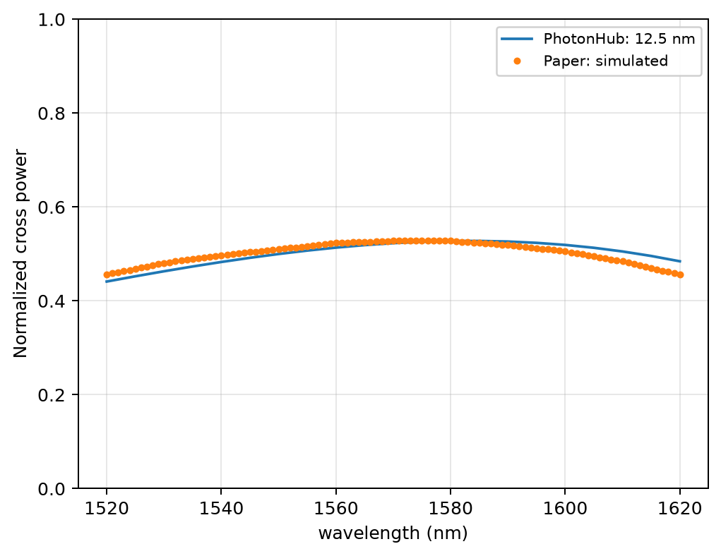
The paper series is its simulated result, extracted from Fig. 4a using the corrected version 2 data. The extraction uncertainty is 0.05 dB.

Result note: the maximum difference from the paper is 2.8161 percentage points; convergence is not established. Full analysis and settings.

Run or adapt this example

Download the source package and unpack it into a PhotonHub source checkout with the recorded compatible SDK and solver. The package contains run.py, the geometry parameters in specs/chen2017_curved_coupler.yaml, and execution instructions. Inspect the mesh size and estimated compute requirements before starting a new run:

python benchmarks/replicate/chen2017_curved_coupler/run.py estimate \
  --label my_curved_coupler --dl .0125 --time-ps 2 \
  --n-freqs 21 --padding 1 --pml .6 --field

Change the width, gap or bend radius in the parameter file to explore a new coupler. Keep the input and both output monitors so the same power normalization applies. Follow the package's execution instructions and use a new run label. These recorded scripts require a compatible SDK and solver; compatibility with later versions is not established. Raw field outputs are not included in the compact source package.

Reproduce these plots

For the spectra alone, save the plotting script, 12.5 nm result data and paper reference in one folder. With PhotonHub and Matplotlib installed, run:

python plot_transmission.py

This uses ph.viz.plot_comparison to replot the saved result. It does not run a simulation. The source and analysis downloads identify any omitted operational metadata in their public manifests; the numerical results are unchanged.

Reference: Chen et al., Scientific Reports (2017), doi:10.1038/s41598-017-07618-6, Fig. 4a. Curves were extracted from vector artwork and converted from dB to normalized power. Replotted under CC BY 4.0.