Deterministic photonic-crystal nanobeam cavity

A nanobeam cavity is a silicon waveguide, a narrow strip that guides light, with a row of holes etched through it. A periodic row of holes is a Bragg mirror: each hole reflects a little, and within a band of wavelengths the reflections add up and turn the light back. Two such mirrors facing each other trap light between them in about a cubic wavelength, which makes nanobeams compact filters, lasers and sensors. The difficulty is where the mirror begins: if the holes start abruptly, the trapped field changes too sharply and scatters out of the beam. The quality factor Q measures how long the cavity stores light; it is the resonance wavelength divided by the resonance's width. Good designs usually come from a long search over hole sizes. A deterministic recipe needs no search: a constant period, no gap between the mirrors, and holes that shrink linearly away from the centre, so the mirror strength grows gradually and the field fades smoothly. Designs reach a simulated Q of a million or more; fabrication roughness brings measured values down to tens of thousands.

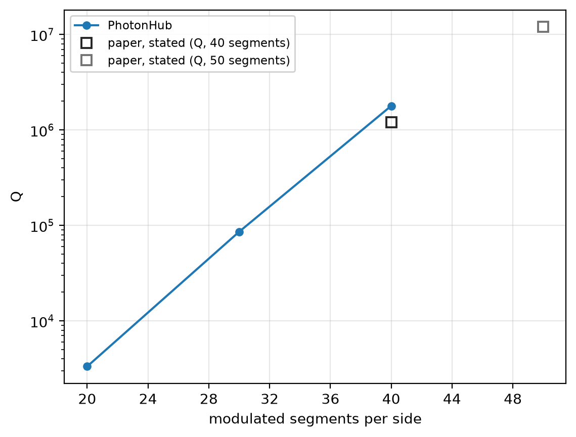
This notebook rings down the cavity "mod40" of Quan, Deotare and Loncar, Appl. Phys. Lett. 96, 203102 (2010), with 40 tapered segments on each side: resonance 1540.0 nm against the paper's 1552 nm, Q 1.8 × 10⁶ against 1.2 × 10⁶. Mirrors of 20 and 30 segments show how Q grows with the mirror length.

Parameters

The design numbers and indices are the paper's, then its stated results. The period is 310 nm, not the paper's rule of thumb of about 300 nm: at 310 nm the band edge of the central segment, the edge of its reflecting band, sits at the 1525 nm design wavelength, the paper's design condition. The mesh is uniform, a whole fraction of the period, so every hole meets the grid alike. The 10 ps ring-down is about a hundredth of the photon lifetime: it pins the resonance and reads Q to about 10 % to 20 %. The pulse reaches a resonance anywhere within 2 % of 1525 nm. The PML sits 0.8 µm from the silicon, and the mode's three mirror planes cut the run to one eighth.

import matplotlib.pyplot as plt
import numpy as np

import photonhub as ph
from photonhub.analysis import ResonanceAnalysis, select_resonances

# design, the paper's Table I and design steps
wlen0 = 1.525  # design wavelength (µm)
a = 0.310  # period (µm); sets the band edge at wlen0
w = 0.700  # nanobeam width (µm)
t = 0.220  # silicon thickness (µm)
n_si = 3.46  # silicon index, constant
n_clad = 1.45  # silica above, below and in the holes
ff_center = 0.15  # hole filling fraction beside the centre
ff_end = 0.0  # filling fraction of the outermost segment
segments = 40  # modulated segments per side, "mod40"
paper_wlen_nm = 1552.0  # paper, Table I: mod40 resonance (nm)
paper_q = 1.2e6  # paper, Table I: mod40 Q
paper_q_mod50 = 1.2e7  # paper, Table I: mod50 Q
mod50 = 50  # paper, mod50: segments per side

# simulation choices
cells_per_a = 8  # uniform mesh cells per period
sides = 96  # corners of each hole polygon
record_ps = 10.0  # ring-down recorded (ps)
fwidth_hz = 1e13  # pulse bandwidth (Hz)
feed = 1.0  # plain waveguide past the last segment (µm)
clearance = 0.8  # silica between the beam and the PML (µm)
pml = 12  # PML layers
symmetry = (1, -1, 1)  # the mode's three mirror planes
samples_per_period = 16  # probe samples per optical period
sweep = [20, 30]  # shorter mirrors, segments per side

f0 = ph.c0 / (wlen0 * 1e-6)  # design frequency (Hz)
wlen = wlen0 * np.linspace(0.98, 1.02, 41)  # profile wavelengths (µm)

Geometry

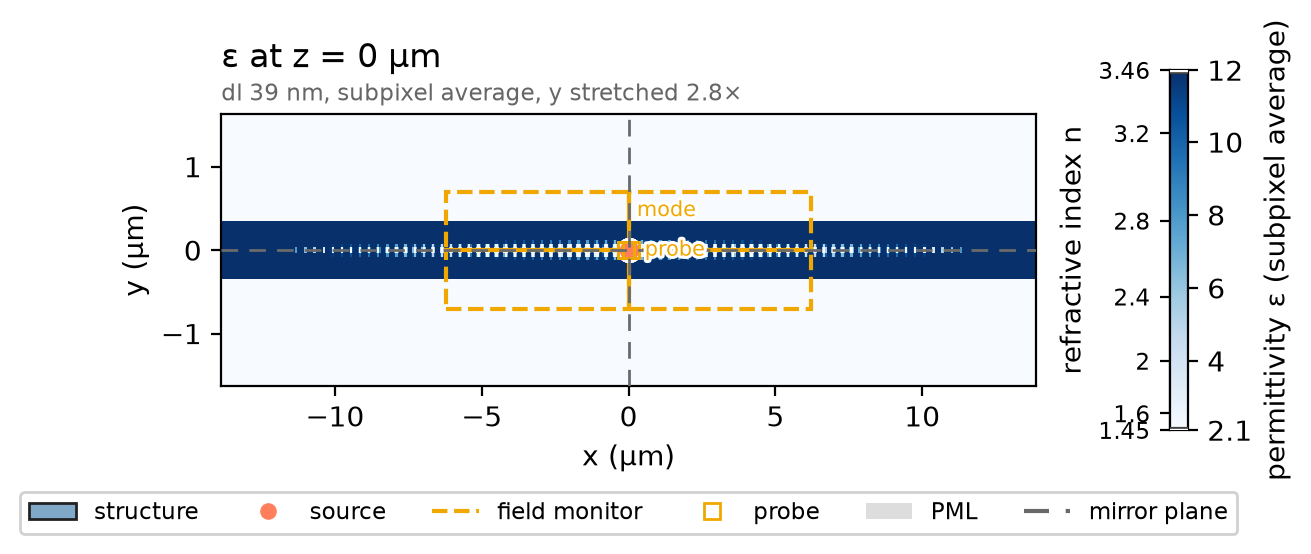
One silicon ph.Box runs through the whole domain. Each segment holds a silica hole, a 96-sided ph.Polygon of area ff * a * w extruded through the silicon (slab_bounds_um), with ff falling linearly from ff_center beside the centre to ff_end; the innermost holes sit one period apart. ph.Medium takes a permittivity, the index squared. holes(n) draws n segments per side, so the mirror length can be swept.

si = ph.Medium(permittivity=n_si**2)
silica = ph.Medium(permittivity=n_clad**2)
length = 2 * (segments * a + feed)  # both mirrors and their feeds (µm)
beam = ph.Structure(
    geometry=ph.Box(center_um=(0.0, 0.0, 0.0), size_um=(2 * length, w, t)), medium=si
)
phi = np.linspace(0, 2 * np.pi, sides, endpoint=False)  # polygon corner angles


def holes(n):
    # the silica holes of n segments per side, ff falling linearly from the centre
    ff = [ff_center + (ff_end - ff_center) * m / (n - 1) for m in range(n)]
    r = [np.sqrt(2 * f * a * w / (sides * np.sin(2 * np.pi / sides))) for f in ff]
    return [
        ph.Structure(
            geometry=ph.Polygon(
                axis="z",
                vertices_um=[(s * (m + 0.5) * a + r[m] * np.cos(p), r[m] * np.sin(p)) for p in phi],
                slab_bounds_um=(-t / 2, t / 2),
            ),
            medium=silica,
        )
        for m, f in enumerate(ff)
        if f > 0
        for s in (-1, 1)
    ]


structures = [beam] + holes(segments)

Simulation

A y-polarised ph.PointDipole at the centre, driven by a short ph.GaussianPulse, rings the cavity. With no ports, there is no mode window to size. A ph.TimeMonitor probe a quarter period beside it records the field against time, about 16 times per optical period, a step count set by the solver's time step. A ph.ProfileMonitor on the silicon mid-plane records the mode across 2 % around 1525 nm; its ph.Apodization opens after the pulse.

pulse = ph.GaussianPulse(freq0_hz=f0, fwidth_hz=fwidth_hz)
source = ph.PointDipole(center_um=(0.0, 0.0, 0.0), polarization="Ey", source_time=pulse)
dl = a / cells_per_a  # the cell along x, y and z (µm)
dt = 0.99 * dl * 1e-6 / (ph.c0 * np.sqrt(3))  # the time step that cell sets (s)
interval = max(1, int(round(1 / (f0 * samples_per_period * dt))))  # steps per sample
probe = ph.TimeMonitor(
    name="probe", center_um=(a / 4, 0.0, 0.0), fields=("Ey",), interval_steps=interval
)
t_start = 2 * pulse.source_end_time_s  # the pulse is over (s)
apodization = ph.Apodization(
    start_s=t_start, end_s=record_ps * 1e-12 - 2 * t_start, width_s=0.5 * t_start
)
mode = ph.ProfileMonitor.plane(
    "mode",
    "z",
    0.0,
    size_um=(segments * a, 2 * w, 0.0),
    center_um=(0.0, 0.0, 0.0),
    wlens_um=wlen,
    fields=("Ex", "Ey", "Ez"),
    apodization=apodization,
)

ph.Simulation holds the setup. ph.Domain fixes the length along the beam and the clearance to the PML around it; the beam runs on into the PML at both ends. ph.Mesh(dl_um=...) sets the uniform cell, with subpixel averaging at the hole walls. The run records a fixed ring-down with no early stop.

sim = ph.Simulation(
    domain=ph.Domain(extent_um=(length, None, None), clearance_um=clearance),
    mesh=ph.Mesh(dl_um=dl),
    background=silica,
    pml_num_layers=pml,
    symmetry=symmetry,
    structures=structures,
    sources=[source],
    monitors=[probe, mode],
    run=ph.RunSpec(run_time_s=record_ps * 1e-12, shutoff=0.0),
    wlen0_um=wlen0,
)
sim.plot_index(z=0.0)
plt.show()

ph.run_local runs the solver on this computer; ph.cloud.run_quoted runs it on a cloud GPU.

data = ph.run_local(sim, quiet=True)
# On a cloud GPU instead, with GPU and SOLVER from your closed-test guide:
# data = ph.cloud.run_quoted(sim, device=GPU, solver=SOLVER)

Field

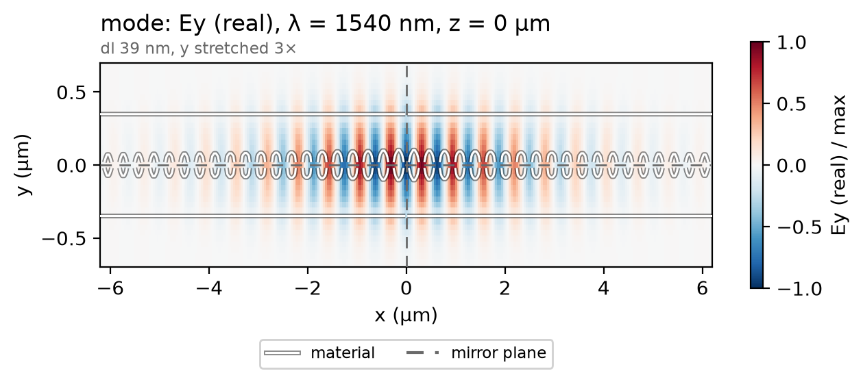
The cavity rings where its geometry puts it, so the profile is read at the recorded wavelength holding the most field. Ey changes sign from one period to the next, peaking in the silicon between the holes, under an envelope that fades smoothly into both mirrors, as the taper was designed to make it.

total = np.abs(data["mode"]).sum(("component", "x", "y", "z"))  # |E| summed per wavelength
f_map = float(total.idxmax("f"))  # the recorded frequency nearest the resonance (Hz)
data.plot_field("mode", field="Ey", z=0.0, freq=f_map)
plt.show()

Result

The resonance and Q come from fitting the decaying poles of the probe's ring-down after the pulse, within 6 % of the design frequency.

def fit(run):
    # (resonance in nm, Q) of the strongest decaying pole within 6 % of f0
    band = (0.94 * f0, 1.06 * f0)
    ringdown = {"probe": run["probe"].sel(t=slice(t_start, record_ps * 1e-12))}
    poles = ResonanceAnalysis(freq_window=band, init_num_freqs=120).run(ringdown, "probe")
    top = select_resonances(poles, freq_window=band, require_decay=True, sort_by="amplitude")
    top = top.isel(freq=0)
    return ph.c0 / float(top.coords["freq"].values) * 1e9, float(top["Q"].values)


resonance, q = fit(data)
print(
    f"resonance {resonance:.1f} nm (paper: {paper_wlen_nm:.0f} nm, designed for "
    f"{wlen0 * 1e3:.0f} nm) | Q {q:.2g} (paper: {paper_q:.2g})"
)

output

resonance 1540.0 nm (paper: 1552 nm, designed for 1525 nm) | Q 1.8e+06 (paper: 1.2e+06)

The recipe's lever is the mirror length: more segments make the taper gentler, so less light leaks. The same beam with 20 and 30 segments per side, in the same domain, rings down and is fitted the same way. The squares are the paper's stated Q for 40 and 50 segments.

qs = []
for n in sweep:
    run = ph.run_local(sim.with_changes(structures=[beam] + holes(n), monitors=[probe]), quiet=True)
    qs.append(fit(run)[1])
ph.viz.plot_comparison(
    sweep + [segments],
    qs + [q],
    stated=[
        (segments, paper_q, "paper, stated (Q, 40 segments)"),
        (mod50, paper_q_mod50, "paper, stated (Q, 50 segments)"),
    ],
    xlabel="modulated segments per side",
    ylabel="Q",
    yscale="log",
)
plt.show()
print(" | ".join(f"{n} segments: Q {v:.2g}" for n, v in zip(sweep + [segments], qs + [q])))

output

20 segments: Q 3.3e+03 | 30 segments: Q 8.6e+04 | 40 segments: Q 1.8e+06

At 8 cells per period the resonance reads 1540.0 nm; at 20 cells per period, 1542.4 nm, not shown converged; the paper's 3D FDTD, 1552 nm. The run uses a uniform 38.75 nm mesh, subpixel averaging on, constant indices of 3.46 and 1.45, 12 PML layers and three mirror planes.