Shape-optimized waveguide taper

A photonic chip carries light in waveguides, silicon strips that hold light by total internal reflection. Light travels along one as modes, field patterns that keep their shape; circuits use the simplest, TE0. A taper joins a narrow waveguide to a wide one, such as a 0.5 µm waveguide to a grating coupler that sends light to a fibre. If the width grows quickly, TE0 cannot keep up: part of the light turns into higher-order modes or leaves the guide. A linear taper must be adiabatic, so gradual that the mode adapts, which takes hundreds of micrometres. Shape optimization instead moves the vertices of a short taper's outline to raise its transmission T, the fraction of the power reaching the wide guide's TE0. One simulation gives T; a second, the adjoint, gives the derivative of T with respect to every vertex. The figure of merit is T, or 10 log₁₀ T in decibels (dB); a good taper loses under 0.1 dB.

This notebook optimizes the 18 µm long, 0.5 to 9 µm taper of Michaels and Yablonovitch, Opt. Express 26, 31717 (2018) in 2D: T rises from 0.4978 for the linear taper to 0.99229 (-0.034 dB), against the paper's 0.51 and just over 0.99 (-0.041 dB).

Parameters

As in the paper, the model is 2D: the 220 nm silicon slab becomes a core of index n_core, the index the slab's TE0 travels with (its effective index), which the paper does not state. The mesh is the paper's 25 nm. Every run lasts exactly n_steps, with no early stop, so the gradient is exact for the T each run computes.

import matplotlib.pyplot as plt
import numpy as np
from scipy.optimize import minimize

import photonhub as ph
from photonhub.analysis import mode_launch, solve_mode_on_cross_section

# design, the paper's symbols (Sec. 4)
L = 18.0  # taper length (µm)
w_in = 0.5  # input guide width (µm)
w_out = 9.0  # output guide width (µm)
n_vertices = 200  # vertices on the taper's top edge
R0 = 0.15  # smallest radius of curvature wanted (µm)
wlen0 = 1.55  # wavelength (µm)
n_core = 2.847485541364588  # assumed: TE0 index of the 220 nm Si slab
n_clad = 1.444  # SiO2 index
paper_start_T = 0.51  # paper, stated linear taper T
paper_final_T = 0.99  # paper, stated final T (just over)
paper_final_db = -0.041  # paper, stated final T (dB)
paper_iterations = 97  # paper, stated iterations to the stop

# simulation choices: the mesh and the run
dl = 0.025  # uniform mesh step, the paper's grid (µm)
pml = 12  # PML layers (0.3 µm)
n_steps = 12000  # fixed run length, no early stop
fwidth = 0.1  # pulse bandwidth, as a fraction of f0

# where things sit (µm)
x_src = 1.0  # source plane, from the input wall
x_in = 1.5  # input port, from the input wall
lead = 2.0  # input wall to the taper's narrow end
past = 1.5  # output port, past the taper's wide end
tail = 2.8  # taper's wide end to the output wall
through = 1.0  # guides run on past each wall
reach = 1.0  # fixed polygon end in the wide guide, past the taper's wide end
overhang = 0.2  # design region past each taper end
margin = 0.3  # design region beside the wide guide, in y
clearance = 1.0  # oxide in y from design region to PML
half_in = 1.5  # narrow guide's mode window, half-width in y
half_out = 5.5  # wide guide's mode window, half-width in y

# the optimizer
pad = 2  # fixed vertices added at each chain end
alpha = 0.01  # assumed: penalty per vertex sharper than R0
kappa = 50.0  # assumed: penalty sharpness (1/µm)
dx_max = 0.04  # largest x move, under half the vertex spacing (µm)
gap = 0.05  # closest a vertex comes to axis or edge (µm)
ftol = 1e-4  # stop when the merit changes less (paper)
gtol = 1e-12  # no stop on a small gradient

f0 = ph.c0 / (wlen0 * 1e-6)  # frequency (Hz)

Geometry

The optimizer's pixels, one per mesh cell, have faces a quarter cell off the cell boundaries, clear of every field sample. pixel_face puts the guide axis and the taper's ends on such faces, so guides and pixels line up.

# helpers that place things on the mesh, whose cells are dl wide
def round_to_cells(length):  # rounded to a whole number of cells (µm)
    return round(length / dl) * dl


def pixel_face(x):  # a quarter cell past the cell boundary nearest x (µm)
    return (round(x / dl) + 0.25) * dl


def cell_centre(x):  # half a cell past the nearest cell boundary (µm)
    return (round(x / dl) + 0.5) * dl


size_x = round_to_cells(lead + L + tail)  # domain length, PML included (µm)
size_y = round_to_cells(2 * (w_out / 2 + margin + clearance + pml * dl))  # domain width (µm)
yc = pixel_face(size_y / 2)  # the guide axis (µm)
x_start = pixel_face(lead)  # the taper's narrow end (µm)
x_end = pixel_face(lead + L)  # its wide end (µm)
x_in_port = cell_centre(x_in)  # where the input port is placed (µm)
x_out_port = cell_centre(lead + L + past)  # where the output port is placed (µm)

guide builds a straight guide on the axis, a ph.Box that ph.Structure fills with the core index.

def guide(x_from, x_to, width):  # a straight guide on the axis
    box = ph.Box(
        center_um=(0.5 * (x_from + x_to), yc, 0.5 * dl),
        size_um=(x_to - x_from, width, 3 * dl),  # z: through the one cell and past it
    )
    return ph.Structure(geometry=box, medium=ph.Medium(permittivity=n_core**2))


guide_in = guide(-through, x_start, w_in)  # from past the input wall, through the PML, to the taper
guide_out = guide(x_end, size_x + through, w_out)  # from the taper, through the PML, past the wall
# no taper: for the launched power and the modes of the source and the input port
straight = guide(-through, size_x + through, w_in)

The design is the taper's top edge, n_vertices points mirrored about the axis; the parameters are their x and y moves. ph.DesignRegion holds the pixels the optimizer may change. ph.PolygonProfile sets each pixel to the fraction of its area inside the polygon. A vertex moved a nanometre then changes the permittivity a little instead of flipping a pixel, so a gradient method can move edges on a fixed grid. pad_ends adds fixed vertices on the guides so the curvature penalty below sees where the taper meets them.

region_length = L + 2 * overhang  # along x (µm)
region_width = w_out + 2 * margin  # across, in y (µm)
region = ph.DesignRegion.on_grid(
    center_um=((x_start + x_end) / 2, yc, 0.0),  # centred on the taper
    size_um=(region_length, region_width, 2 * dl),  # z: two cells, around the one simulated cell
    dl_um=dl,
    shape=(round(region_length / dl), round(region_width / dl), 1),  # a pixel per cell in x and y
    eps_min=n_clad**2,  # an empty pixel is oxide
    eps_max=n_core**2,  # a full one is core
    merge_boxes=True,  # fewer boxes for the solver to set up
)
edge_x = np.linspace(x_start, x_end, n_vertices)  # the top edge's vertices
edge_y = yc + w_in / 2 + (w_out - w_in) / 2 * (edge_x - x_start) / L  # on the linear taper
first = (x_src, yc + w_in / 2)  # a fixed vertex in the narrow guide; any x before the region does
last = (x_end + reach, yc + w_out / 2)  # and one inside the wide guide
taper = ph.PolygonProfile(
    region=region,
    vertices_um=(first, *zip(edge_x, edge_y), last),
    movable=tuple(range(1, n_vertices + 1)),  # all but first and last
    mirror=("y", yc),  # the bottom edge mirrors the top
).pad_ends(spacing_um=edge_x[1] - edge_x[0], count=pad)
p0 = np.zeros(taper.num_params)  # no vertex moved: the linear taper

Simulation

ph.Simulation holds the setup: a uniform dl grid, oxide background, PML on the x and y walls, and one periodic cell along z, which makes the run 2D.

sim = ph.Simulation(
    size_um=(size_x, size_y, dl),  # one cell along z: a 2D run
    grid=ph.UniformMesh(dl_um=dl),
    run=ph.RunSpec(n_steps=n_steps, shutoff=0, dft_shutoff=0),  # no early stop
    background=ph.Background(permittivity=n_clad**2),  # oxide
    boundaries=ph.Boundaries(x="pml", y="pml", z="periodic"),
    pml_num_layers=pml,
    subpixel=False,  # the gradient needs it off; the polygon is area-averaged per pixel instead
)

te0_mode solves one guide's TE0 mode on this grid with solve_mode_on_cross_section. Its electric field lies in the chip plane; the paper calls the same mode TM, with the magnetic field Hz out of the plane.

def te0_mode(waveguide, x, half_width):  # TE0 of one guide alone, on the plane x
    return solve_mode_on_cross_section(
        sim.with_changes(structures=[waveguide]),
        axis="x",
        plane_value_um=x,
        wlen_um=wlen0,
        pol="TE",  # E in the chip plane: the paper's TM
        mode_index=0,  # the fundamental mode
        h_center_um=yc,  # on the guide axis
        v_center_um=0.0,
        half_w_um=half_width,  # the mode window's half-width
        half_v_um=dl,  # the one cell along z
        dl_um=dl,
        supersample=1,  # the guide as the solver samples it
    )


mode_src = te0_mode(straight, x_src, half_in)  # launched by the source
mode_in = te0_mode(straight, x_in_port, half_in)  # read at the input port
mode_out = te0_mode(guide_out, x_out_port, half_out)  # read at the output port

A ph.TransmissionPort is a plane across a guide where a mode is read; readout, a ph.ModeTransmission between the two, gives their monitors.

port_in = ph.TransmissionPort(
    mode=mode_in,
    axis="x",
    position_um=x_in_port,
    out_direction="-",  # pointing away from the taper
    name="input",
    center_um=(yc, 0.0),  # (y, z) of the guide axis
)
port_out = ph.TransmissionPort(
    mode=mode_out,
    axis="x",
    position_um=x_out_port,
    out_direction="+",  # pointing away from the taper
    name="output",
    center_um=(yc, 0.0),
)
# the ports' monitors here, and below the launched amplitude for objective
readout = ph.ModeTransmission(input_port=port_in, output_port=port_out, freq_hz=f0)
ports = readout.monitors(sim)  # the two port planes as monitors

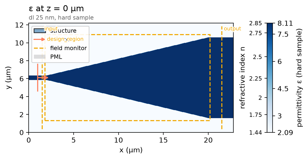
mode_launch sends a TE0 pulse around f0 into the narrow guide. The design region's monitor records the field the gradient needs. The plot shows the start, the linear taper's pixels rho0.

pulse = ph.GaussianPulse(freq0_hz=f0, fwidth_hz=fwidth * f0)
source = mode_launch(
    sim,
    mode_src,
    axis="x",
    position_um=x_src,
    source_time=pulse,
    direction="+",  # toward the taper
    center_um=(yc, 0.0),
)
design_field = region.monitor(f0, simulation=sim)  # the field over the region
rho0 = taper.density(p0)  # the linear taper as pixel densities
sim = sim.with_changes(
    sources=tuple(source),
    structures=(guide_in, guide_out, *region.structures(rho0)),
    monitors=(design_field, *ports),
)
sim.plot_index(z=0.0)
plt.show()

One run of no_taper, the straight guide alone, gives the launched power; objective, the T to raise, divides by it.

no_taper = sim.with_changes(structures=(straight,), monitors=ports)  # straight guide, ports only
reference = ph.run_local(no_taper, quiet=True)
objective = ph.ModeTransmission(
    input_port=port_in,
    output_port=port_out,
    freq_hz=f0,
    # the launched amplitude, held fixed so a reflection off the taper cannot change it
    incident_amplitude=readout.reference_incident_amplitude(reference),
)

The optimizer raises the merit: T minus a curvature penalty, about alpha for each vertex bent well tighter than R0. The paper gives the penalty's form but not alpha or kappa, and the penalty is not a fabrication check. Each call of merit is a forward and an adjoint run, giving T and its derivative for all 400 vertex moves (ph.parametric_value_and_gradient).

def build(rho):  # the simulation with the region's pixels at densities rho
    return sim.with_changes(structures=(guide_in, guide_out, *region.structures(rho)))


def merit(p):  # minus the merit (T minus the penalty) at p, and its gradient: SciPy minimizes
    evaluation = ph.parametric_value_and_gradient(
        build_forward=build,
        region=region,
        objective=objective,
        p=p,
        expand=taper.density,  # vertex moves to pixel densities
        jacobian=taper.jacobian,  # and their exact derivative
        # test that derivative on the first call only, while T_evals (made in the next
        # cell) is empty: the test re-renders the polygon along every parameter
        check_jacobian=len(T_evals) == 0,
    )
    penalty, penalty_grad = taper.curvature_penalty(p, r0_um=R0, alpha=alpha, kappa_per_um=kappa)
    T_evals.append(evaluation.value)
    return -(evaluation.value - penalty), -(evaluation.grad - penalty_grad)

SciPy's L-BFGS-B, a gradient-based optimizer, holds each parameter within bounds that keep the polygon from crossing itself. As in the paper, it stops when the merit changes by less than ftol. This cell takes most of the notebook's run time.

# reset here, so re-running this cell starts a fresh optimization
T_evals = []  # T at each evaluation; an iteration may take several
T_iter = []  # T after each iteration


def after_iteration(p):  # SciPy calls this once per iteration
    T_iter.append(T_evals[-1])  # its last evaluation is the step it took


vertices = taper.chain_um(p0)  # the linear taper's vertices (µm)
bounds = []  # (low, high) per parameter: dx, then dy, of each vertex
for k in taper.movable:
    from_axis = vertices[k, 1] - yc  # the vertex's distance from the axis
    # x moves stay within ±dx_max; y keeps each vertex at least gap from the axis, so from
    # its mirror image, and gap inside the region's edge
    bounds += [(-dx_max, dx_max), (gap - from_axis, w_out / 2 + margin - gap - from_axis)]
result = minimize(
    merit,
    p0,
    jac=True,  # merit returns its gradient too
    method="L-BFGS-B",
    bounds=bounds,
    callback=after_iteration,
    options={"ftol": ftol, "gtol": gtol},
)

Field

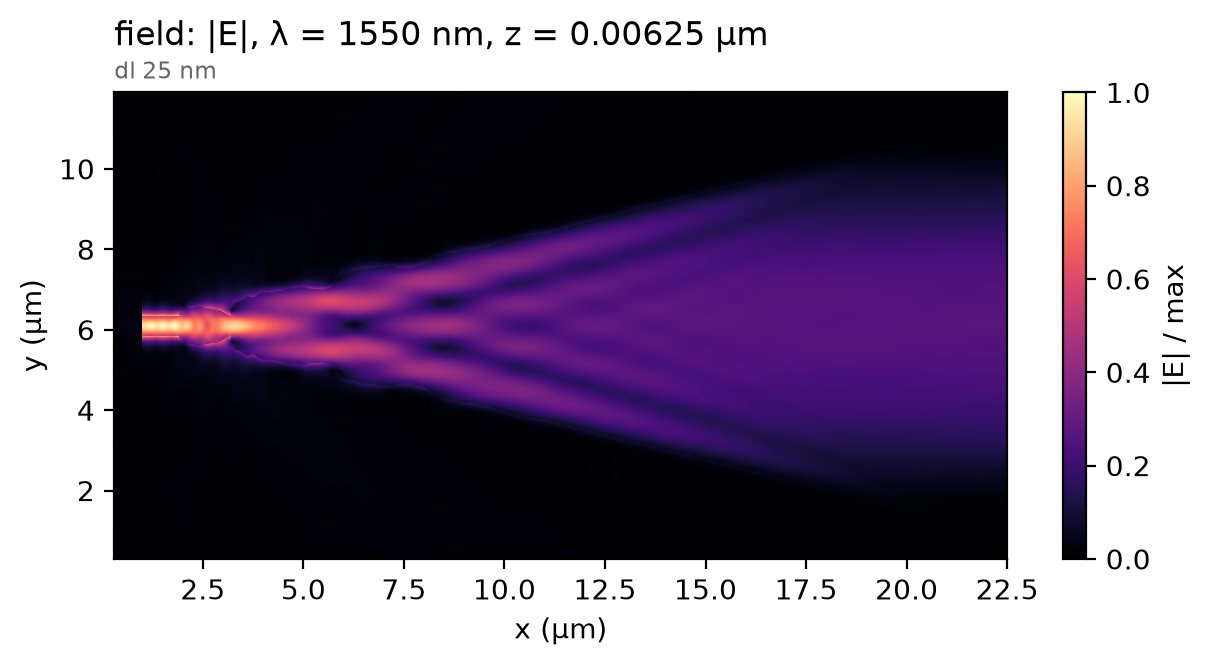
The optimized taper runs once more, recording the field. The light splits into beams that spread and interfere, then reach the wide guide as one broad lobe, its TE0 mode.

field = ph.ProfileMonitor.plane(
    name="field",
    axis="z",
    position_um=dl / 4,  # a quarter cell up: every component records in the one cell
    freqs_hz=[f0],
    fields=("Ex", "Ey", "Ez", "Hz"),  # Hz only for the 3D view's phase
)
rho = taper.density(result.x)  # the optimized taper as pixel densities
optimized = build(rho).with_changes(monitors=(*ports, field))  # ports and the field only
data = ph.run_local(optimized, quiet=True)
data.plot_field("field", field="E", z=dl / 4)
plt.show()

Result

The curve is T after each iteration; iteration 0 is the linear taper. The dashed and dotted lines are the paper's stated final and start values; its licence bars re-plotting its curves, and its BFGS iterations need not match ours one to one.

T = np.array([T_evals[0], *T_iter])  # the linear taper, then each iteration
iterations = np.arange(T.size)  # 0 is the linear taper
ph.viz.plot_comparison(
    iterations,
    T,
    stated=[
        (paper_final_T, "paper, stated (final T)"),
        (paper_start_T, "paper, stated (linear taper T)"),
    ],
    xlabel="iteration",
    ylabel="transmission T",
)
plt.show()
T_db = 10 * np.log10(T[-1])
print(
    f"linear taper T {T[0]:.4f} | optimized T {T[-1]:.5f} ({T_db:.3f} dB) after {result.nit} "
    f"iterations | paper: just over {paper_final_T} ({paper_final_db} dB) after {paper_iterations}"
)

output

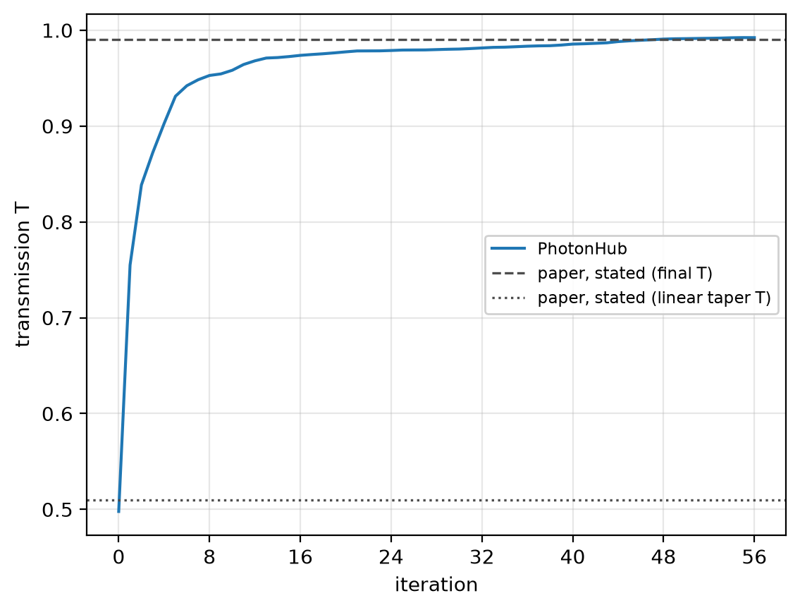
linear taper T 0.4978 | optimized T 0.99229 (-0.034 dB) after 56 iterations | paper: just over 0.99 (-0.041 dB) after 97

On the uniform 25 nm mesh, T reads 0.99229 at 1550 nm; converged, 0.9921, for this design at 10 nm; the paper's frequency-domain method, just over 0.99. The linear taper's 0.4978 falls to 0.4931 at 10 nm. The run stops on the paper's rule, not at an optimum. The 25 nm run uses the 2D model, area-averaged pixels, subpixel averaging off, non-dispersive indices, 12 PML layers and no symmetry plane.