Nanopost metasurface lens

A lens focuses light by delaying it more at its centre than at its edge, so that every path reaches the focus in step; a glass lens does it with a curved surface, which is thick and hard to make small. A metasurface lens is flat: a single layer of posts shorter than the wavelength, standing on glass. Each post acts as a tiny waveguide, and its diameter sets the phase, the delay, of the light it transmits; posts whose diameters follow the lens's phase profile focus the light, and one lithography step makes the whole lens. The numerical aperture (NA), between 0 and 1, says how steeply a lens bends light toward its focus; a high NA gives a small spot but is hard to reach, because the rim posts must bend the light most. Three numbers rate it: the transmission, the share of the light that passes; the focusing efficiency, the share that reaches the focal spot, typically 0.4 to 0.9; and the spot's full width at half maximum (FWHM), in wavelengths (λ), down to about 0.5 λ.

This notebook builds the amorphous-silicon lens of Arbabi et al., Nat. Commun. 6, 7069 (2015) as a 50 µm lens of NA 0.89 from the paper's post library, lights it with the paper's fibre beam and reads the focal spot: focusing efficiency 0.718 against the paper's stated 3D FDTD 0.72; transmission 0.797 against 0.85, spot 0.63 λ against 0.68 λ.

Parameters

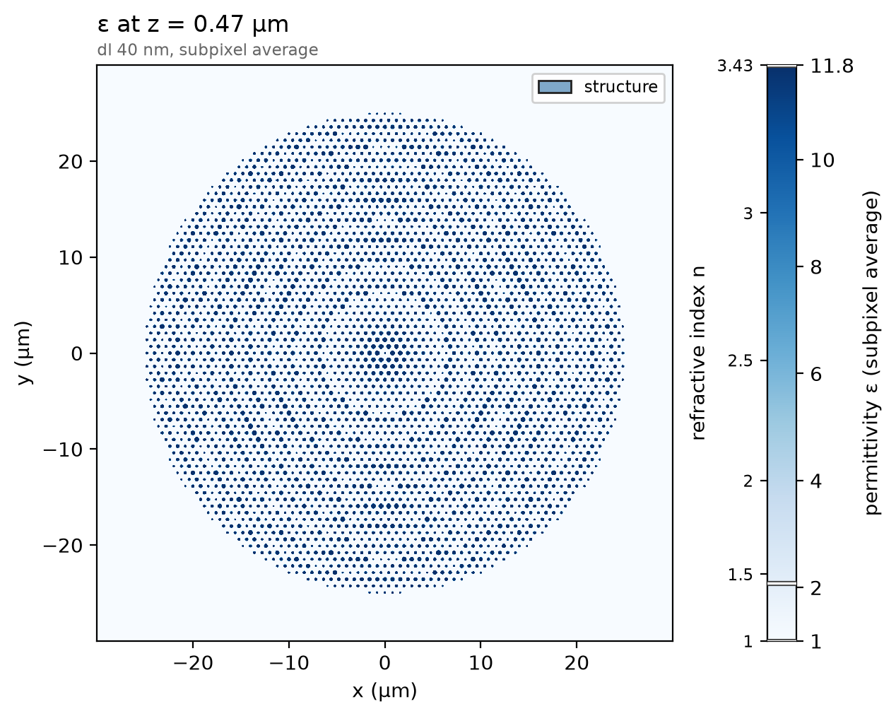
The design numbers are the paper's, then its stated results for this NA. The paper simulated a 100 µm lens; this one is 50 µm, the focusing distance scaled to keep the NA. The beam is a standard single-mode fibre's output after 150 µm of air and 125 µm of silica, scaled with the lens. It matters: under a plane wave the validation study reads an efficiency of 0.40, because the rim posts are then fully lit. The mesh has 40 nm cells; the lens's periodic copy sits 5 µm from its rim, where the beam is below 1e-3 of its peak.

import json

import matplotlib.pyplot as plt
import numpy as np

import photonhub as ph
from photonhub.analysis import diffraction_orders, focal_metrics

# design, the paper's symbols
a = 0.800  # hexagonal lattice constant (µm)
h_post = 0.940  # amorphous-silicon post height (µm)
n_asi = 3.43  # a-Si index at 1550 nm (the paper's value)
D_min = 0.200  # smallest post diameter used (µm)
D_max = 0.550  # largest post diameter used (µm)
D_lens = 50.0  # lens diameter (µm); the paper simulated 100
d_focus = 12.5  # focusing distance (µm): NA 0.89
w_beam = 12.37  # fibre beam 1/e field radius at the lens (µm)
paper_fwhm = 0.68  # paper, stated 3D FDTD spot at NA 0.89 (λ)
paper_transmission = 0.85  # paper, stated 3D FDTD transmission
paper_efficiency = 0.72  # paper, stated 3D FDTD focusing efficiency

# simulation choices
wlen0 = 1.550  # design wavelength (µm), the one read out
cells_per_wlen = 11.3  # mesh cells per wavelength in a-Si: 40 nm
sub = 0.5  # substrate kept below the posts (µm)
clearance = 1.0  # air above the posts (µm)
pad = 5.0  # lens rim to its periodic copy (µm)
pml = 12  # PML layers
run_fs = 686  # longest run (fs): the pulse and its ring-down
shutoff = 1e-6  # field decay that ends the run
dft_shutoff = 0.0  # 0 = no spectrum-settling check
n_scan = 31  # planes scanned for the focus
cut_half = 4.0  # half-width of the focal cut shown (µm)

f0 = ph.c0 / (wlen0 * 1e-6)  # design frequency (Hz)

Geometry

The lens is centred on the origin and stands on z = 0, the top of the substrate. Its post library is the paper's Fig. 1d table of transmitted phase against post diameter, read from its reference file, without the resonance band the paper excludes.

tab = json.load(open("refs/arbabi2015_fig1d.json"))  # the paper's Fig. 1d
D_tab = np.array(tab["series"]["phase_over_2pi"]["x"]) / 1e3  # post diameter (µm)
phi_tab = 2 * np.pi * np.array(tab["series"]["phase_over_2pi"]["y"])  # its phase (rad)
lo, hi = np.array(tab["excluded_diameter_range_nm"]) / 1e3  # the resonance band (µm)
use = (D_tab >= D_min) & (D_tab <= D_max) & ((D_tab < lo) | (D_tab > hi))
D_tab, phi_tab = D_tab[use], phi_tab[use]

The design rule is the paper's: the hyperbolic phase for a focus at d_focus, sampled at every lattice site inside the lens, each site given the post whose tabulated phase is closest.

rows = int(D_lens / (a * np.sqrt(3))) + 2  # lattice rows that cover the lens
sites = [
    (a * (i + j / 2), a * np.sqrt(3) / 2 * j)
    for j in range(-rows, rows + 1)
    for i in range(-2 * rows, 2 * rows + 1)
]
sites = [(x, y) for x, y in sites if np.hypot(x, y) <= D_lens / 2]  # inside the lens
phi = [-2 * np.pi / wlen0 * (np.sqrt(x**2 + y**2 + d_focus**2) - d_focus) for x, y in sites]
D = [D_tab[np.argmin(np.abs(np.angle(np.exp(1j * (phi_tab - p)))))] for p in phi]  # closest phase

Each post is a ph.Cylinder along z; ph.Medium takes the a-Si index as a permittivity, and ph.Structure pairs each shape with its medium. The substrate is the background, and an air ph.Box fills the space above it.

period = D_lens + 2 * pad  # the lens and its padding, repeated
z_top = h_post + clearance  # the wall above the posts
air = ph.Structure(
    geometry=ph.Box(
        center_um=(0.0, 0.0, (z_top + clearance) / 2),
        size_um=(period + 2 * clearance, period + 2 * clearance, z_top + clearance),
    ),
    medium=ph.Medium(permittivity=1.0),
)
posts = [
    ph.Structure(
        geometry=ph.Cylinder(
            axis="z", center_um=(x, y, h_post / 2), radius_um=d / 2, length_um=h_post
        ),
        medium=ph.Medium(permittivity=n_asi**2),
    )
    for (x, y), d in zip(sites, D)
]
structures = [air] + posts
print(f"{len(posts)} posts, diameters {min(D) * 1e3:.0f} to {max(D) * 1e3:.0f} nm")

output

3559 posts, diameters 200 to 528 nm

Simulation

The fibre beam is a ph.GaussianBeam launched inside the substrate with a flat phase front: the paper's beam arrived curved and its lens's phase undid the curvature, so a flat beam on the plain hyperbolic phase is the same pair. Its waist is eight wavelengths wide, so it launches as its sampled profile (paraxial=True). There are no ports: two ph.ProfileMonitor planes record the tangential fields over one period, in just above the beam for the launched power and field above the posts, the transmitted plane the focus is computed from.

beam = ph.GaussianBeam(
    "z",
    -sub / 2,
    waist_um=w_beam,
    polarization="Ex",
    center_um=(0.0, 0.0, 0.0),
    paraxial=True,
)
inward = ph.ProfileMonitor.plane(
    "in", "z", -sub / 4, wlens_um=wlen0, fields=("Ex", "Ey", "Hx", "Hy")
)
field = ph.ProfileMonitor.plane(
    "field",
    "z",
    h_post + clearance / 2,
    wlens_um=wlen0,
    fields=("Ex", "Ey", "Ez", "Hx", "Hy"),
)

ph.Simulation holds the setup. ph.Domain is one period across, periodic along x and y (ph.Boundaries), with PML above and below; ph.Mesh is uniform at cells_per_wlen cells per wavelength in the a-Si, with subpixel averaging at the post walls.

sim = ph.Simulation(
    domain=ph.Domain(period_um=(period, period, None), extent_um=(None, None, (-sub, z_top))),
    mesh=ph.Mesh(cells_per_wlen=cells_per_wlen, uniform=True),
    background=ph.materials.SiO2,  # the substrate
    boundaries=ph.Boundaries(x="periodic", y="periodic", z="pml"),
    pml_num_layers=pml,
    structures=structures,
    wlens_um=wlen0,
    source=beam,
    run=ph.RunSpec(run_time_s=run_fs * 1e-15, shutoff=shutoff, dft_shutoff=dft_shutoff),
    monitors=[inward, field],
)
sim.plot_index(z=h_post / 2)
plt.show()

ph.run_local runs the solver on this computer; ph.cloud.run_quoted runs it on a cloud GPU. The outputs on this page come from a GPU run of this exact simulation.

data = ph.run_local(sim, quiet=True)
# On a cloud GPU instead, with GPU and SOLVER from your closed-test guide:
# data = ph.cloud.run_quoted(sim, device=GPU, solver=SOLVER)

Field

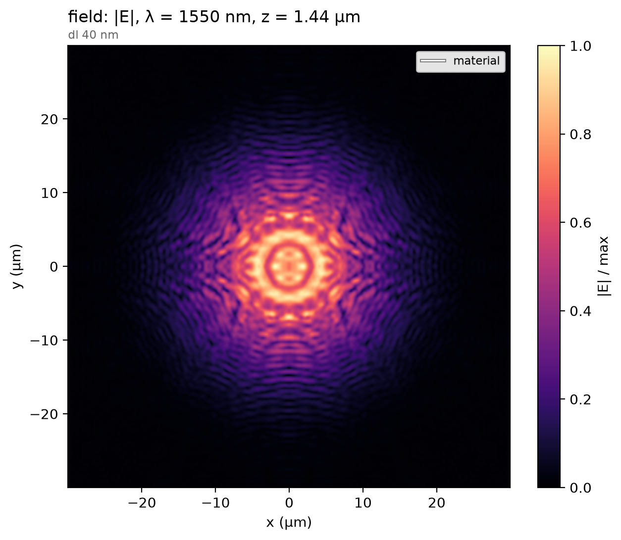
The transmitted field just above the posts: the beam, now carrying the hyperbolic phase, with the post-by-post modulation the lattice imprints.

data.plot_field("field", field="E", z=h_post + clearance / 2)
plt.show()

Result

diffraction_orders reads the forward power through in, which everything is normalised by. focal_metrics propagates the recorded plane to the focus as a sum of plane waves, finds the plane of peak flux and reads, by the paper's definitions, the FWHM of a 2-D Gaussian fit, the transmission and the focusing efficiency, the power within three FWHM of the axis. The square marks the paper's stated FWHM at half maximum; its licence does not allow re-plotting its curves.

P_in = float(diffraction_orders(sim, data, "in").power_forward.sum())  # launched power
focus = focal_metrics(
    sim,
    data,
    "field",
    dz_um=np.linspace(0.5 * d_focus, 1.5 * d_focus, n_scan),
    incident_power=P_in,
    disc_radius_um=D_lens / 2,
    center_um=(0.0, 0.0),
)
x_um, cut = focus.focal_cut
sel = np.abs(x_um) <= cut_half
ph.viz.plot_comparison(
    x_um[sel],
    cut[sel],
    stated=(paper_fwhm * wlen0 / 2, 0.5, "paper, stated (FWHM)"),
    xlabel="x (µm)",
    ylabel="normalized flux at the plane of focus",
)
plt.show()
print(
    f"focus {focus.z_peak_um + clearance / 2:.1f} µm past the posts | "
    f"FWHM {focus.fwhm_um / wlen0:.3f} λ (paper {paper_fwhm}) | "
    f"transmission {focus.transmission:.3f} (paper {paper_transmission}) | "
    f"focusing efficiency {focus.efficiency:.3f} (paper {paper_efficiency})"
)

output

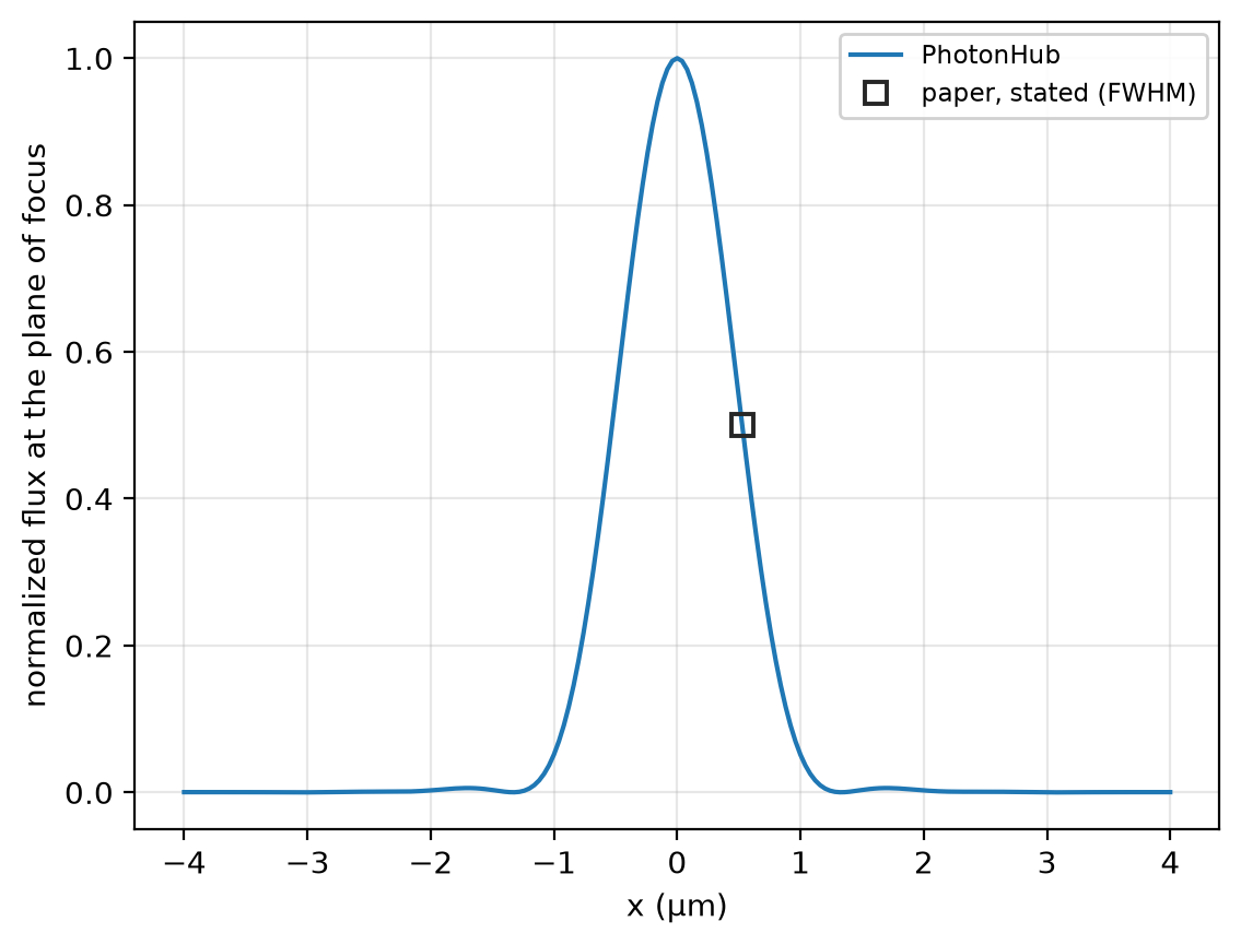
focus 12.3 µm past the posts | FWHM 0.631 λ (paper 0.68) | transmission 0.797 (paper 0.85) | focusing efficiency 0.718 (paper 0.72)

At 11.3 cells per wavelength the focusing efficiency reads 0.718 at 1550 nm, the only mesh run on this lens, not shown converged; the paper's 3D FDTD, 0.72. The run uses a uniform mesh of 40 nm cells, subpixel averaging on, non-dispersive a-Si, silica and air, 12 PML layers above and below, periodic walls around the lens and no symmetry plane.