Topological valley transport around sharp bends
A valley photonic crystal guides light along the wall between two honeycomb lattices whose hole sizes are swapped. The wall carries light around sharp 120° corners, where an ordinary photonic-crystal waveguide reflects. This page builds the silicon-on-insulator crystal of He et al., Nat. Commun. 10, 872 (2019) from its published dimensions and computes what three interfaces transmit from 1320 to 1570 nm: straight, a Z with two 120° bends, and an Ω with four. Averaged over the 1360 to 1492 nm band gap the transmission reads straight -2.18 dB, Z-shape -2.72 dB, Ω-shape -3.29 dB, so against the straight wall the Z-shape costs 0.54 dB and the Ω-shape costs 1.11 dB. The recorded runs used 26.6 minutes of GPU time in total.
Recorded study
The figures come from saved simulation results; building this page runs no FDTD. Mesh convergence is not established, and these are simulated values, not measurements.
Download Python Recorded spectra
| Parameter | Value |
|---|---|
| Lattice / hole diameters | 385 nm honeycomb / 81 and 181 nm |
| Silicon thickness / index | 220 nm / 3.47 on oxide 1.45 |
| Crystal / access guides | 23 lattice constants x 27 rows (8.9 x 9.0 um) / 1.7 um strips |
| Interfaces | straight, Z (two 120 deg bends), Omega (four) |
| Mesh | 20.3 x 18.5 nm in plane (19 per lattice constant, 18 per row), 18.3 nm in the silicon |
| Subpixel smoothing | volume-average permittivity |
| Boundaries | 16 PML layers on every face; oxide through the wall |
| Band / duration | 1320-1570 nm, 126 wavelengths / 5 ps, 138,151 steps |
The whole study is one script against the PhotonHub Python API. Download it at the top of the page and run it to reproduce every figure here.
import numpy as np
import matplotlib.pyplot as plt
from matplotlib.path import Path
import photonhub as ph
from photonhub.analysis import mode_launch, mode_monitor, solve_mode_on_cross_section
Build the crystal
The design is the published one: a 385 nm honeycomb lattice of 81 nm and 181 nm air holes in 220 nm silicon on oxide, fed by 1.7 µm strips. Each interface is a chain of bearded domain walls written as a heading and a row index, and a 120° turn keeps the wall bearded. The empty path is a plain strip, the reference every spectrum is divided by. The crystal is 23 lattice constants long and 27 rows tall, the published 9 × 9.2 µm² footprint.
# Design (µm): lattice constant, the two hole diameters, silicon thickness, strip width.
a, d1, d2, t, w = 0.385, 0.081, 0.181, 0.220, 1.700
n_si, n_sio2 = 3.47, 1.45
# Each interface is a chain of bearded cut lines: (heading in degrees, row index).
paths = {"strip": [],                 # no crystal: the straight strip the spectra are normalized to
         "flat": [(0, 0)],
         "Z": [(0, 0), (240, 14), (0, -6)],
         "Omega": [(0, 0), (120, -8), (0, 6), (240, 15), (0, 0)]}
n_len, n_rows = 23, 27                # crystal: lattice constants long, rows tall
facet_holes = True                    # keep the holes centred on the crystal's two end faces
band, n_lam = (1.320, 1.570), 126       # wavelength band (µm) and points
lam_map, show = 1.430, "Z"            # field map: Fig. 2e's wavelength and interface
# Simulation choices.
cells_x, cells_y = 19, 18             # cells per lattice constant and per row spacing
access, clear_xy, clear_z = 1.6, 0.5, 0.8
pml, record_ps = 16, 5.0
smoothing = "volume"                   # subpixel operator: volume-average permittivity in boundary cells
Silicon (n = 3.47), air and oxide (n = 1.45) are lossless and nondispersive, the published values.
si = ph.Medium(permittivity=n_si ** 2)
air = ph.Medium(permittivity=1.0)
sio2 = ph.Medium(permittivity=n_sio2 ** 2)
The mesh is commensurate with the lattice: 19 cells per lattice constant along x and 18 per row along y (20.3 and 18.5 nm, about 20 cells per wavelength in silicon and under the 24 nm the design was published at), so every hole is meshed the same way. A mesh laid out per wavelength instead would place each hole differently on the grid, which scatters light along the wall like disorder. Along z it is 18.3 nm in the silicon and grades to 46 nm in the claddings. Sixteen PML layers close every face.
h = a * np.sqrt(3) / 2                # row spacing
dx, dy = a / cells_x, h / cells_y
dz_si = t / (2 * int(np.ceil(t / (2 * min(dx, dy)))))
dz_max = min(band) / (n_sio2 * 20)
steps, dz = [], dz_si
while sum(steps) < clear_z:
    dz = min(1.25 * dz, dz_max)
    steps.append(dz)
steps += [dz_max] * pml               # outward from the silicon
z_steps = steps[::-1] + [dz_si] * round(t / dz_si) + steps
z_nodes = tuple(float(round(z, 9)) for z in np.r_[0.0, np.cumsum(z_steps)][:-1])
z_lo = sum(steps)
zc = z_lo + t / 2
nx = round((n_len * a + 2 * access) / dx) + 2 * pml
ny = round((n_rows * h + 2 * clear_xy) / dy) + 2 * pml
size = (nx * dx, ny * dy, sum(z_steps))
x0 = round((pml * dx + access) / dx) * dx
grid = ph.GradedMesh(dl_um=dx, coords=ph.GradedMeshAxis(
    y=tuple(round(j * dy, 9) for j in range(ny)), z=z_nodes))
The crystal is one honeycomb lattice. A hole's size depends only on its sublattice and on which side of the interface path it sits, so the two big holes facing each other across every wall leave a 41 nm silicon bridge, the published spacing. The crystal's two end faces pass through hole centres and those holes are kept, as in the published layout: whole holes where a strip lands, half holes along the rest of each face. Silicon strips butt onto the crystal on the wall, the island is etched around, and the oxide runs through the PML.
def crystal(lines):
    """Substrate, silicon and holes for one interface path; an empty path is the plain strip."""
    solid = [ph.Structure(medium=sio2, geometry=ph.Box(center_um=(size[0] / 2, size[1] / 2, 0.0),
                                                        size_um=(2 * size[0], 2 * size[1], 2 * z_lo)))]
    if not lines:
        strip = ph.Box(center_um=(size[0] / 2, size[1] / 2, zc), size_um=(size[0] + 2, w, t))
        return solid + [ph.Structure(medium=si, geometry=strip)], size[1] / 2, size[1] / 2
    normal = lambda deg: np.array([-np.sin(np.radians(deg)), np.cos(np.radians(deg))])
    offset = lambda m: (m - 1 / 6) * h
    corners = [np.linalg.solve([normal(p), normal(q)], [offset(i), offset(j)]) for (p, i), (q, j) in zip(lines, lines[1:])]
    ys = [offset(lines[0][1]), offset(lines[-1][1])] + [c[1] for c in corners]
    mid = (min(ys) + max(ys)) / 2
    y0, far = round((size[1] / 2 - mid) / dy) * dy, 10 * size[0]
    upper = Path(np.array([(-far, ys[0]), *corners, (far, ys[1]), (far, far), (-far, far)]) + [x0, y0])
    holes = []
    for m in range(-2 * n_rows, 2 * n_rows):
        for n in range(-2 * n_len, 3 * n_len):
            for y, big_above in ((m * h, True), (m * h + 2 * h / 3, False)):
                x = n * a + m * a / 2
                inside = -1e-9 < x < n_len * a + 1e-9 if facet_holes else 0 < x < n_len * a
                if inside and abs(y - mid) < n_rows * h / 2:
                    d = d2 if upper.contains_point((x0 + x, y0 + y)) == big_above else d1
                    holes.append(ph.Structure(medium=air, geometry=ph.Cylinder(
                        axis="z", center_um=(x0 + x, y0 + y, zc), radius_um=d / 2, length_um=t)))
    y_in, y_out = y0 + ys[0], y0 + ys[1]
    island = ph.Box(center_um=(x0 + n_len * a / 2, y0 + mid, zc), size_um=(n_len * a, n_rows * h, t))
    strips = [ph.Box(center_um=(x0 / 2, y_in, zc), size_um=(x0 + 2 * dx + a / 2, w, t)),
              ph.Box(center_um=((x0 + n_len * a + size[0]) / 2, y_out, zc), size_um=(size[0] - x0 - n_len * a + 2 * dx + a / 2, w, t))]
    return solid + [ph.Structure(medium=si, geometry=g) for g in [island] + strips] + holes, y_in, y_out
Launch and read out
A Gaussian pulse covers 1320 to 1570 nm, read at 2 nm steps. Cells cut by a hole's edge take the volume-average permittivity (smoothing), the operator that places this crystal's pass band where the published transport calculation has it; the last section gives the size of that choice. Recording runs for 5 ps unless the field decays to 10⁻⁶ of its peak first; the crystal legs used the full 5 ps.
c0 = 299792458.0
lam = np.linspace(*band, n_lam)
freqs = tuple(float(c0 / (value * 1e-6)) for value in lam)
f0 = 0.5 * (freqs[0] + freqs[-1])
f_map = c0 / (lam_map * 1e-6)
pulse = ph.GaussianPulse.for_band(wavelengths_um=list(band), freq0_hz=f0)
scene = dict(size_um=size, grid=grid, background=ph.Background(permittivity=1.0),
             boundaries=ph.Boundaries(x="pml", y="pml", z="pml"), pml_num_layers=pml,
             subpixel=True, subpixel_method=smoothing)
run = ph.RunSpec(run_time_s=record_ps * 1e-12, shutoff=1e-6)
TE₀ of the input strip is launched 0.4 µm beyond the PML, in the simulation interior, and measured 0.4 µm downstream. Transmission is the Poynting flux through the whole output plane over the incident TE₀ power. Dividing that by the plain strip's own ratio removes the launch and the readout, leaving what the crystal does.
window = dict(half_w_um=w / 2 + 0.8, half_v_um=t / 2 + 0.6, v_center_um=zc, dl_um=dx)
x_src, x_out = pml * dx + 0.4, size[0] - pml * dx - 0.4
sims, mon = {}, {}
for shape, lines in paths.items():
    structures, y_in, y_out = crystal(lines)
    basis = ph.Simulation(**scene, run=run, structures=tuple(structures))
    mode_in = solve_mode_on_cross_section(basis, "x", x_src, lam_map, "TE", 0, h_center_um=y_in, **window)
    mode_out = solve_mode_on_cross_section(basis, "x", x_out, lam_map, "TE", 0, h_center_um=y_out, **window)
    source = mode_launch(basis, mode_in, axis="x", position_um=x_src, source_time=pulse, direction="+")
    mon[shape] = {"in": mode_monitor(basis, mode_in, axis="x", position_um=x_src + 0.4, freqs_hz=freqs, name="in"),
                  "out": mode_monitor(basis, mode_out, axis="x", position_um=x_out, freqs_hz=freqs, name="out")}
    flux = ph.PowerMonitor(name="flux_out", axis="x", position_um=x_out, freqs_hz=freqs)
    field = ph.ProfileMonitor(name="field", center_um=(size[0] / 2, size[1] / 2, zc),
                              size_um=(size[0] - 2 * dx, size[1] - 2 * dy, 0.0),
                              fields=("Ex", "Ey", "Ez"), freqs_hz=(f_map,), interval_space=(2, 2, 1))
    planes = tuple(m.field_monitor for m in mon[shape].values()) + (flux,) + ((field,) if lines else ())
    sims[shape] = ph.Simulation(**scene, run=run, structures=tuple(structures),
                                sources=tuple(source), monitors=planes)
The setup figure shows the Z-shape interface's permittivity at the silicon mid-plane, with the source and the monitor planes.
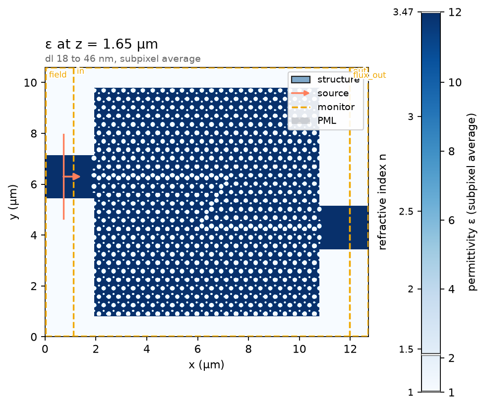
Relative permittivity at the silicon mid-plane, with the mode source (line), the monitor planes (dashed) and the absorbing boundaries.
Run it
Inspect the estimate before starting a run. It covers one crystal leg at the full recording length.
cost estimate: $0.81 (4.063 Tcell-steps @ $0.2/Tcell-step)
  grid     : 627 x 572 x 82 = 29,408,808 cells, 138,151 steps (dt = 3.619e-17 s)
  memory   : 2.0 GiB resident (device), 331.7 MiB output
  walltime : ~3.4 min @ 20 Gcells/s (full duration; auto-shutoff may finish sooner)
This cell starts the four simulations, the strip and the three interfaces, when you run the downloaded script. It was not executed to build this page; the figures below come from the recorded runs.
Field profile
At 1430 nm, inside the band gap, the field stays on the domain wall: straight across, around both corners of the Z, and around all four of the Ω. The scale is decibels below each map's own maximum, so the decay into the crystal is visible.
titles = {"flat": "straight", "Z": "Z-shape, two bends", "Omega": "\u03a9-shape, four bends"}
walls = [s for s in data if s != "strip"]
fig, axes = plt.subplots(len(walls), 1, figsize=(6.6, 3.7 * len(walls)), constrained_layout=True, sharex=True)
for ax, shape in zip(np.atleast_1d(axes), walls):
    data[shape].plot_field("field", field="E", val="abs", z=zc, freq=f_map, simulation=sims[shape],
                           structures=False, scale="db", db_floor=-30, ax=ax)
    ax.annotate(titles[shape], xy=(0.02, 0.03), xycoords="axes fraction", color="white")
plt.show()
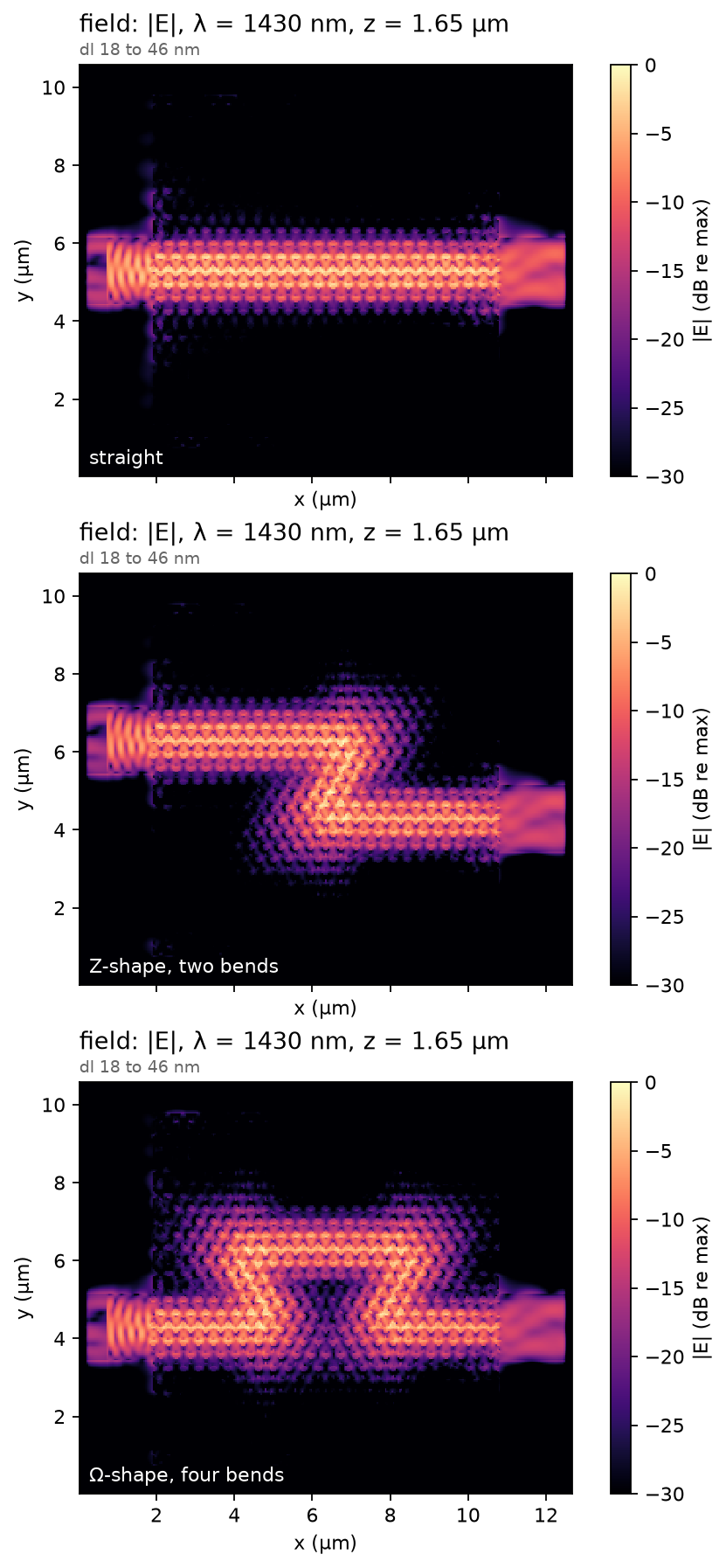
Recorded |E| at 1430 nm on each interface, in decibels below each map's own maximum. The wall guides the light; the crystal around it stays dark.
Transmission
All three interfaces share one axis. Inside the band gap each carries a flat pass band; outside it the crystal rejects, and the bent walls fall off earlier than the straight one at long wavelengths.
T_db = {}
for shape in paths:
    pin = mon[shape]["in"].mode_power(data[shape], direction="+")
    flux = data[shape]["flux_out"].sel(f=list(freqs)).values
    T_db[shape] = 10 * np.log10(flux / np.array([pin[f] for f in freqs]))
T_db = {shape: T_db[shape] - T_db["strip"] for shape in paths if paths[shape]}
ax = ph.viz.plot_comparison(lam * 1e3, T_db["flat"], label="straight", ylabel="transmission (dB)", ylim=(-30, 1))
for shape in [s for s in T_db if s != "flat"]:
    ax.plot(lam * 1e3, T_db[shape], label={"Z": "Z-shape, two bends", "Omega": "\u03a9-shape, four bends"}[shape])
ax.legend()
plt.show()
gap = (lam > 1.360) & (lam < 1.492)
print("mean in the band gap (dB):", {shape: round(float(v[gap].mean()), 2) for shape, v in T_db.items()})
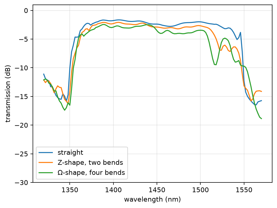
Transmission of the three walls, each divided by the plain strip at the same mesh.
| interface | mean transmission in the band gap | cost of the bends | pass band (−10 dB) | TE₀ reflection in the gap |
|---|---|---|---|---|
| straight | -2.18 dB | reference | 1350 to 1549 nm | 0.046 |
| Z-shape | -2.72 dB | -0.54 dB | 1353 to 1547 nm | 0.050 |
| Ω-shape | -3.29 dB | -1.11 dB | 1354 to 1552 nm | 0.053 |
At 19 cells per lattice constant and 18 per row spacing, the straight interface transmits -2.18 dB on average across the band gap; a converged value is not established. The smoothing operator matters at this mesh: with the default contour operator the same crystal reads -2.34 dB and its pass band runs from 1330 to 1529 nm, against 1350 to 1549 nm here. Volume averaging weights silicon more in every boundary cell, which moves the bands to longer wavelengths by an amount that shrinks with the cell size. The difference between the two operators is the size of the discretization error to expect on these numbers.
Adapt this
- Change
d1andd2to open or close the band gap. - Add a path to
pathsto test another bend sequence. - Refine
cells_xandcells_y, or setsmoothing = "contour", to test convergence.
Validated in: the build record. Every simulation on this page was rebuilt from this recipe and matched the recorded run byte for byte before the figures were drawn.